Pollinator Pollster, Part 7: Up and Running

Pollinator Pollster

This is going to be a technically-focused blog, walking through each major system element in the detection process, which I wanted to cover in detail now that the prototype sensor is 'live' and installed in the garden for data collection trials. I'm going to discuss the pipeline from pollinator detection to the posting of data on the Pi 4 hosted web site to demonstrate the functioning of the system. There will be one final blog post after this, in which I'll share the domain name at which you will also be able to access this site and see the functioning of the sensor yourself.

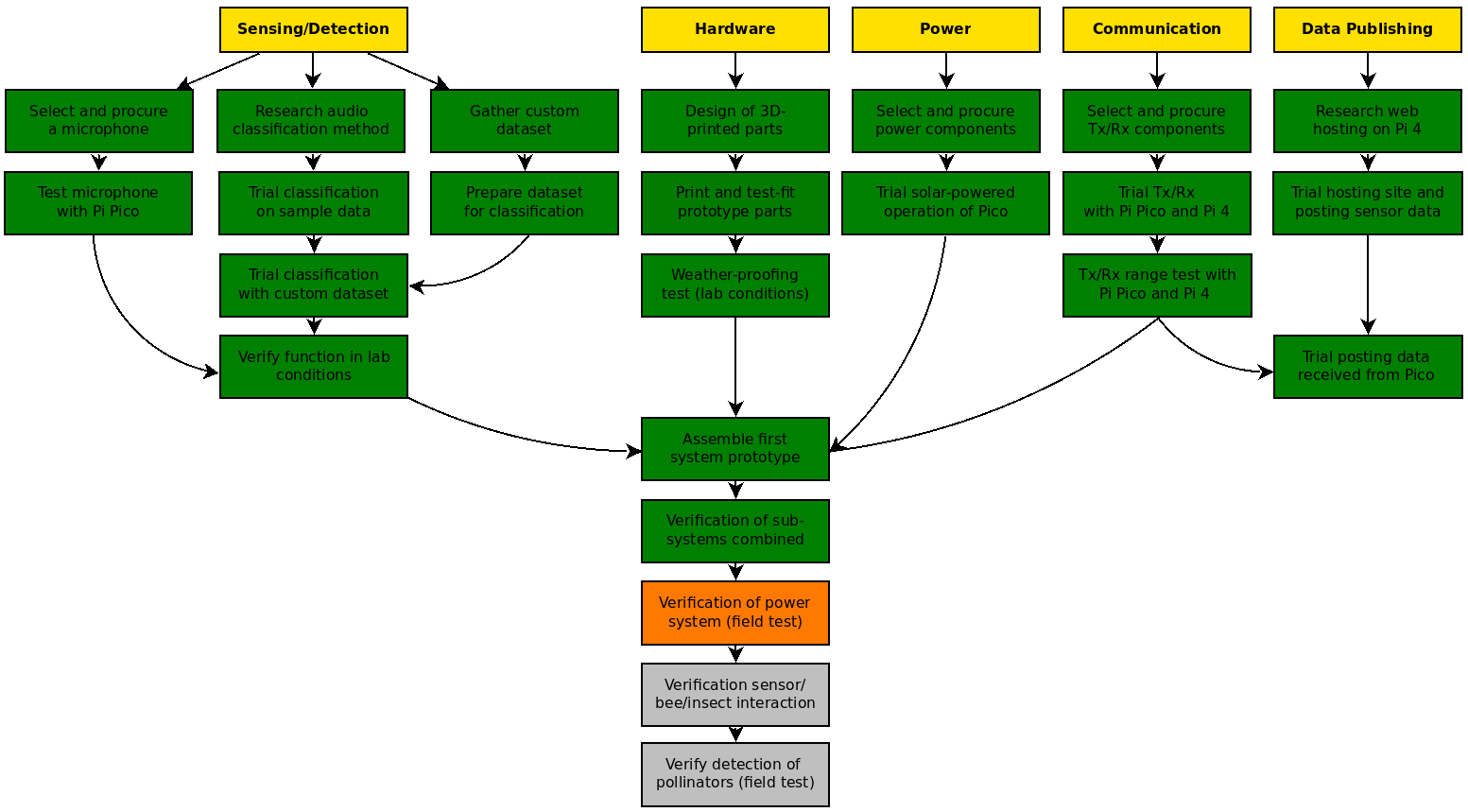
Project Plan

The last time posting the project plan; at this point in time the full system prototype has been brought together, and is now deployed outside, so therefore over the next few days will validate the function of the power system, detection algorithm, and radio system. It has been a very busy few days getting it this far!

Deploying the Sensor

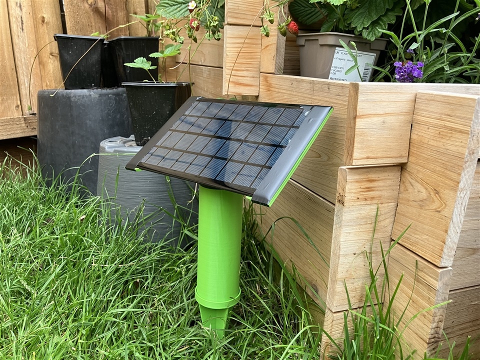
Here's the sensor pictured outside where it will remain from now! It has sprouted a little electrical tape around some of the major joins - although it passed the 'rain test' (garden hose) as you'll remember from the previous blog post, I want to be absolutely sure that no stray raindrop puts a stop to the final testing. There are plenty of plants in flower nearby and a lot of insect traffic, so plenty of opportunities to test correct detection.

Now, let's step through the sensor process which it will be running:

Step 1: The Microphone Detects the Bee

As mentioned before, for the prototype of the system I am using the 'Buff-Tailed Bumblebee', Bombus terrestris, a species I commonly see in my garden, as the example. The microphone, a Sparkfun Analog MEMS microphone, picks up the sound of the bee, perhaps as it visits a nearby flower.

Step 2: Fast Fourier Transform

The incoming audio data (in analog form from the microphone) is then received by the Raspberry Pi Pico for processing. At this stage, the C++ code applies a Fast Fourier Transform (FFT), a method which converts the audio signal from being mapped against the time domain to against the frequency domain. From this, it can be determined the frequency distribution of the data, and also the dominant frequency (the frequency with the greatest sound intensity). The code to do this on the Pi Pico was developed by Alex Wulff (see his blog on hackster 'ADC Sampling and FFT on Raspberry Pi Pico') which I employ to deliver the maximum frequency component.

There are three parameters within Alex's code which can be tuned to adapt the performance of the FFT to specific purpose. I iteratively tested these values with the Pico, whilst using a tone generator app on my phone to create test signals which could be analysed. Those parameters were:

• CLOCK_DIV: The Pi Pico's RP2040 chip has two 'Phase-Locked Loop' circuits, which generate a 48MHz clock signal. The CLOCK_DIV variable divides that by the set number (optimum found to be 9600) into smaller divisions in order to reduce the sampling rate. 48,000,000 / 9,600 = 5,000Hz. The reason for doing so is we aren't interested in higher frequencies than this, so we can focus on the lower range, with greater resolution.
• FSAMP: this needs to be set to the sampling rate to match CLOCK_DIV, so in this case 5000 (Hz).
• NSAMP: this defines the number of samples which will be used for the FFT analysis. A higher value results in greater resolution and detail of the frequency spectrum, but is slower to calculate. A value of 2000 for this was found to be a good compromise, resulting in a frequency resolution of 2.5Hz (adequate to determine if the dominant frequency detected is that of a bee or not), and a satisfactorily fast sampling rate.

I've included a short video below showing testing of the FFT code using a tone generator app, and then 'in the wild' of my garden and the local park, collecting audio samples from bumblebees to determine what the detection criteria should be.

Edit media

Dimensions x Small Medium Large Custom

Subject (required) Brief Description Tags (separated by comma) Video visibility in search results Visible Hidden

Parent content

Pollinator Pollster, Part 7: Up and Running

Poster

Upload Preview

Ok

Cancel

Step 3: Detection Algorithm

Now the FFT code has assigned the dominant frequency within the processed sample to the max_freq variable, the below snippet shows how that is handled. Firstly, to help with debugging and testing, the max_freq value is printed to the Serial. I used this (as shown in the above video) to determine that a dominant frequency of 37.5Hz is observed when this species of bumblebee is present next to the sensor.

Secondly, an if statement is used to determine if the max_freq value falls within a set range. As mentioned above, I believe that a dominant frequency of 37.5Hz indicates the presence of this bee species, hence a range of 35 to 40Hz is used as the test. I use a range rather than an ==37.5 test, as I may need to adjust the lower and upper bounds of this range if it seems I am getting false negatives or false positives.

If the max_freq value passes this test, the detection variable is set to equal 1. This variable is used as a latched test of whether or not a bee has been detected within this time window (see the next step). The variable can only be set back to 0 when this data is sent, hence if a bee is detected within the 5 minute window the detection variable will remain equal to 1, indicating a positive detection. This approach is used (rather than reporting how many detections occurred within the time window, as an individual bee may be detected multiple times, and that would lead to a very misleading count. Instead, the code as is will show at which times of day, and on which days within the year bees are active (in the vicinity of the sensor), an approach which I think would be more useful to a researcher.

Step 4: Data Transmission

The next step of the process is to get that data out of the sensor and to the hub! The code snippet below is a section of the C++ code running on the Pi Pico which handles this operation, so let's look at that in more detail.

At the start of the code snippet, the clock function is used to create a variable called 'elapsedTime'. This is a measure used to create an interval of 5 minutes (or 300 seconds), which is tested for in the first if statement. The purpose of this is to trigger data transmission at 5 minute intervals (rather than constant transmission). The nested if statement then determines whether the HC-12 transceiver sends a '1' if there has been a detection within the previous 5 minute window, or a '0' if not.

Before concluding the if statement, the detection variable is reset to 0, and the startTime variable is now set to match the last endTime variable. This will ensure that the elapsedTime variable is reset to 0 again, and therefore starts again counting up to 300 seconds at which point the next transmission will be triggered.

Step 5: Data Reception

In Part 3 of this blog series I described using an Arduino to program the HC-12 transceivers. They have their own microcontrollers and memory, and hence will remember the parameters (which define frequency, power, and operating mode) that they are programmed with. Both HC-12 units I purchased were programmed (using my trusty Arduino MEGA) to have matching settings, which also complied with UK radio spectrum laws.

With the HC-12 transceiver for the Pi 4 hub therefore, it was just a matter of getting it plugged in (using the same GPIO pins that I had tested with the Pi 3B in Part 3), and then revisiting the Python program I had created at that point. Sidenote: I was using the Pimoroni Fan Shim with the Pi 4, which is controlled using the UART pins, and although it shouldn't interfere with the operation of anything else connected to the GPIO pins, it turned out to block the function of the HC-12 entirely. This drove me round in circles for a while until I realised this issue wasn't code-based!!

The Python program for the Pi 4 needed minor adaptation to write the incoming data to a .csv file and not just print the results to serial as it had done previously. In addition to outputting the [1/0] signifying detection or not detection, it also appends to each line in the .csv file an output of the time function to give each data line a datetime stamp. This will be essential when it comes to processing the results in the next step!

Step 6: Graphing and Publishing

The data from the sensor has been received by the Pi 4 hub, and saved into a .csv file. Next, a separate process is needed to change this data into the right form to present on the Pi 4-hosted web site, so that a researcher can view the data from anywhere at anytime.

After trialing a few options, I decided to use a separate Python program on the Pi 4, along with matplotlib, to graph the data directly from the .csv file, and save this as an image, which can then be picked up by the HTML files serving the Flask app which runs the server.

I will be sharing the web domain in my next and final post, but for now here's an example chart I made (using dummy data) while developing the Python program and experimenting to see what the most effective type of chart might be.

Until Next Time

As always, thank you very much for reading my posts, I have been enjoying your updates this past week too, I hope I can count myself among those who have finished their projects soon. Good luck with your final steps if you're also finishing things off like me, and see you next time!