Take the Poll | Join our Discussion
Advances in Computer Vision
Cameras are an important piece of many electronic systems, including those used in industrial automation, medical, and security applications. In the past, these systems relied uniformly on the eyes of a human operator, watching screens for unusual imagery. Advances in camera technology and processing power, as well as the software crunching the image data, are enabling machines to take over more of the responsibility in determining what the objects in the video might be.
There are many algorithms capable of recognizing objects in an image or video. Before artificial intelligence became viable, there were also a number of more traditional algorithms being used for tasks like facial recognition. For example, Haar Cascades is a widely used algorithm that applies a series of Haar wavelets (the simplest wavelet form) at various scales and combinations throughout an image, searching for objects. Traditional algorithms are very efficient, and can run in real-time on many embedded devices.
Modern algorithms take advantage of today’s available computational power, and use artificial intelligence (AI) and deep learning to train the software on how to detect objects based on existing datasets. Algorithms based on deep learning can be more accurate, but require a great deal more computing power than traditional algorithms and, as such, they run at a slower speed.
Detecting Objects with Artificial Intelligence
The most common tasks for image processing algorithms are object detection and object classification.
Object classification algorithms process the image and try to determine what type of object exists in the image. Typically, there is only one object that needs to be classified in an image, enabling most object classification algorithms to run relatively quickly, even on a microcontroller, where processing power is limited. An example of object classification is using facial recognition for authentication.
For more information on facial recognition, click here to read element14’s Essentials learning module on Face Applications.
Object detection algorithms examine the image looking for one or more specific types of object, as well as their size and location. Object detection is typically more complex than object classification, and requires more data to train.
One of the first successful techniques that was developed for object detection and classification is R-CNN, or “Region-Based Convolutional Neural Network.”
|
What Is a Convolutional Neural Network? A Neural Network (NN) or Artificial Neural Network (ANN) is an algorithm or series of algorithms that attempts to recognize patterns in a dataset. A Convolutional Neural Network (CNN) is an algorithm that iterates through groups of pixels on images, applying filters to each group. Each filter has a specific purpose, from simple tasks like edge detection to recognizing whole objects, such as eyes and ears. CNNs are effective in recognizing patterns, making them useful for imaging and computer vision applications. |
The R-CNN model has three modules:
- Region Proposal: Determine which regions have interesting data in them, and create bounding boxes for each candidate.
- Feature Extractor: Extract features from each region.
- Classifier: Determine if the features are part of a known class.
R-CNN is straightforward and highly accurate, but can be a slow approach, due to the potential for thousands of bounding boxes to be created. Techniques such as Fast R-CNN and Faster R-CNN have been developed to improve on R-CNN’s processing time.
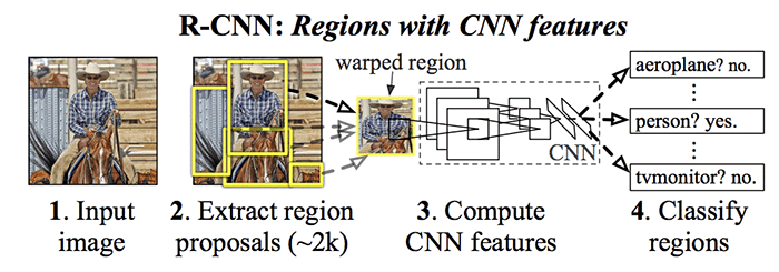
Figure 1: R-CNN Model Architecture
Source: R. Girschick, J. Donahue, T. Darrell, J. Malik, UC Berkeley
YOLO (You Only Look Once) is another family of object recognition models that focuses on fast processing, with the goal of real-time object detection. While R-CNN-based algorithms perform multiple iterations for the same image, YOLO predicts bounding boxes and class probabilities in just one run of the algorithm. It works by splitting an image into a grid, where each cell of the grid is responsible for predicting one or more bounding boxes. A non-maximum suppression (NMS) algorithm is used to select the most accurate bounding boxes for the objects in the image, removing the boxes which were predicted with low certainty. Only the bounding boxes with a high confidence level remain. While YOLO is faster than R-CNN, its accuracy is lower. It might also have trouble detecting multiple objects if they appear in the same grid cell.
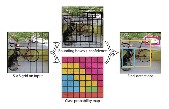
Figure 2: Summary of Predictions Made By the YOLO Model
Source: J. Redmon, S. Divvala, R. GIrshick, A. Farhadi, Univ. Of Washington, Allen Institute for AI, Facebook
SSD (Single-shot Multi-box Detection) is similar to YOLO, in that it divides the image into a grid and detects objects in a single pass. However, their algorithms differ when dealing with multiple bounding boxes of the same instance of an object. Instead of generating multiple bounding boxes and eliminating less accurate ones, SSD starts off first with anchor boxes, or preset boxes of fixed size and aspect ratio, and regresses towards the correct bounding box by calculating confidence loss and location loss. Confidence loss is a measure of how confident the software is that an object exists within the bounding box. Location loss is the distance between the predicted and correct location of the bounding box.
While AI algorithms are evolving to be faster and more efficient, they still require a large amount of computing power and cannot easily run on a microcontroller. Most embedded vision devices rely on traditional algorithms to achieve real-time object detection.
Faster Objects, More Objects
Edge Impulse has introduced a new algorithm called FOMO (Faster Objects, More Objects), which has the efficiency to bring real-time object detection, tracking, and counting to microcontrollers. In some cases, FOMO runs 30 times faster than MobileNet SSD using under 200K of RAM.
One of the underlying concepts of the FOMO algorithm is that the location of the object is more important than the size of the object. After determining the location of the objects, other characteristics can be determined, such as the number of objects and if objects are above or below each other.
Heat Map
FOMO’s neural network architecture consists of a number of convolutional layers. A simple way to visualize these layers is to think of each new layer creating a lower-resolution image of the previous layer. If you start with a 16x16 pixel image, the layers might be:
Layer 1 (Input Layer): 16x16
Layer 2: 4x4 – Each 4x4 block of pixels from Layer 1 is mapped roughly to 1 pixel in Layer 2
Layer 3: 1x1 – The 4x4 image in Layer 2 is mapped down to 1 pixel
The location of objects is roughly preserved as you go deeper; for example, in Layer 2, the pixel at (0, 0) maps to the top left corner of the input image. Naturally, as resolution decreases, the accuracy of the location is reduced as well.
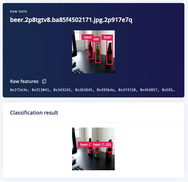
Figure 3: Training on the centroids of beer bottles. The above image shows the annotated training data. The bottom shows the inference result.
Source: Edge Impulse
By default, FOMO creates 8x8 pixel cells to create a per-region class probability map. It then uses a custom loss function, which preserves the location information in the final layer, creating a heat map of where the objects are located in the image. Figure 3 illustrates a heat map generated from a 160x160 pixel input image. The resulting heat map is 20x20, or 8x smaller.
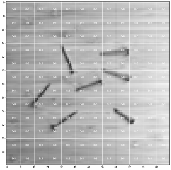
Figure 4: 96x96 image, split into a 12x12 grid
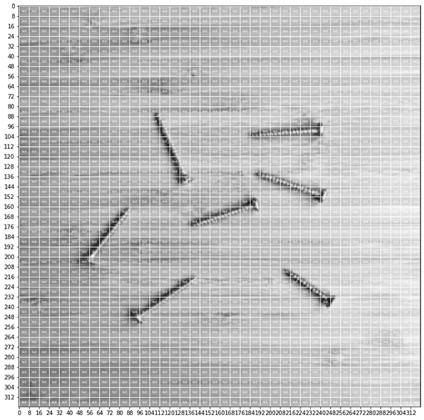
Figure 5: 320x320 image, split into a 40x40 grid
Figures 4 and 5 illustrate images of two different resolutions (96x96 and 320x320), split into grids with 8x8 cells.
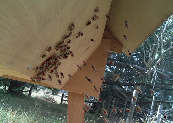
Figure 6: Counting individual bees with an earlier version of FOMO. The size of each cell in the grid was set to 2x2.
The resolution of the grid is configurable. Figure 6 illustrates the effects of increasing the resolution of the grid, giving you the ability to count a large number of small objects due to the pixel-level segmentation.
Because size is no longer a concern, classical bounding boxes are no longer necessary. The FOMO algorithm detects objects based on their center point, or centroid. Counting objects becomes a simple task, because every activation on the heat map is an object. There is no need to dedicate additional computational power towards calculating the size and location of a bounding box. If desired, bounding boxes can be generated by creating boxes around the highlighted areas; however, for many applications, bounding boxes are not required.
Application Example: Car Parking Occupancy Detection with FOMO
To keep track of available spaces, automated occupancy detection systems in parking lots often use sensor networks based on magnetometers, ultrasonic, and infrared sensors, which can be expensive to install and maintain, as well as difficult to scale. A computer vision-based system is a scalable and cost-effective alternative. This reference project is available from Edge Impulse and serves as a tutorial for Edge Impulse Studio and FOMO.
The first step is collecting and annotating images of cars. These are used to train the algorithm. YOLOv5 offers a “car” class, which includes a pre-trained model that can be used as the starting point for training. Annotation can be automated in Edge Impulse Studio, greatly simplifying the process when working with large datasets.
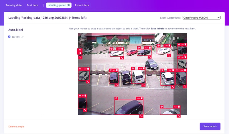
Figure 7: AI-assisted labeling using YOLOv5
Once the dataset is annotated, the training can begin. In Edge Impulse Studio, this consists of setting image parameters, such as resolution and color space, and choosing the model for object detection.
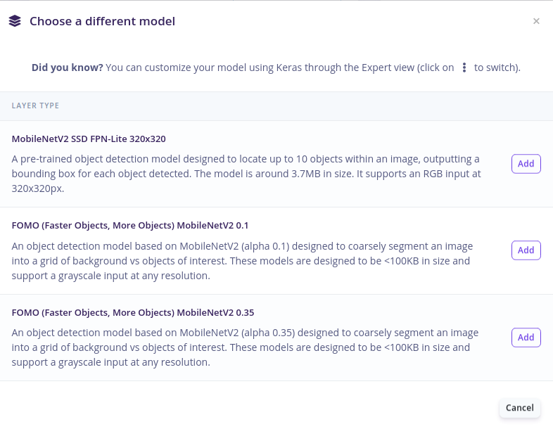
Figure 8: Choosing an object detection model
After training for 100 epochs (one epoch is one cycle through the entire training dataset) at a learning rate of 0.001, the confusion matrix shows the following results.
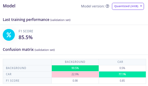
Figure 9: FOMO training results
When the test image was input into the trained FOMO model, 14 cars out of 17 were detected, which is impressive, given the small amount of training images and training cycles. A larger dataset, with more training time, would yield a more accurate count. For the same test image, an SSD MobileNetV2 model with the same amount of training detected 10 cars.
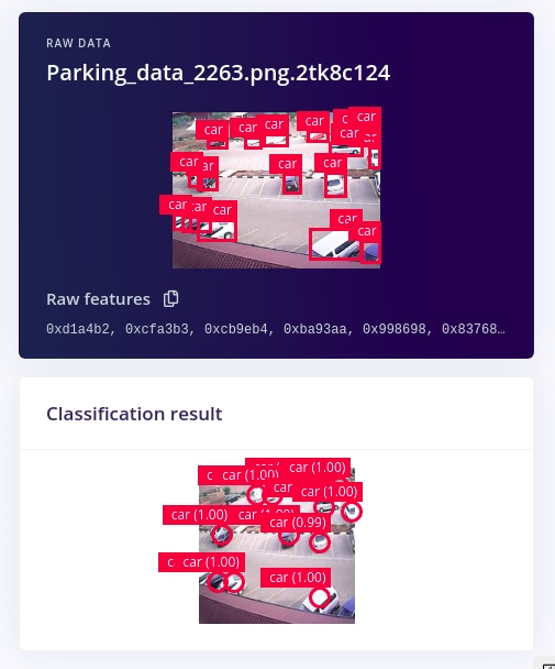
Figure 10: FOMO live classification results
When tested on a Raspberry Pi 4, classification using the FOMO model had a latency of 36ms, corresponding to a framerate of 27.7fps, while SSD MobileNetV2 had a latency of 642ms or a 1.56fps framerate. FOMO used just 77KBs of flash memory and 243.9KBs of RAM. In comparison, SSD MobileNetV2 used 11MB of flash. The speed and low memory usage of FOMO make it well suited for applications running on microcontrollers.
Development Boards
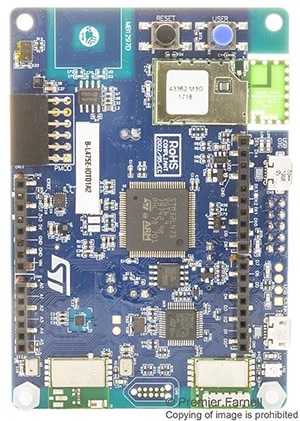
ST IoT Discovery Kit
Buy Now
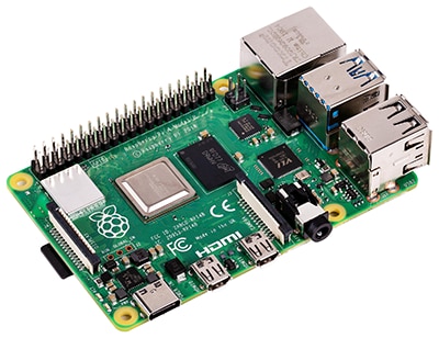
Raspberry Pi 4
Buy Now
Limitations of FOMO
Because FOMO does not invest the processing cycles into determining an object’s size, it is more accurate with applications where objects are a similar size. FOMO is essentially object detection where all bounding boxes are square and with an approximate size of 1/8th the resolution of the input image. Additionally, objects that are too close to each other may not be detected accurately, because their centroids might occupy the same cell. In many cases, however, resolution can be increased to avoid this limitation.
Conclusion
Artificial intelligence algorithms show a great deal of promise for computer vision-based applications; however, they can be slow and processor intensive. Algorithms based on R-CNN, YOLO, and SSD have evolved over time to become more accurate and efficient, but there is room for improvement. FOMO (Faster Objects, More Objects) is an algorithm from Edge Impulse that delivers accurate results at speeds quick enough to run on microcontrollers.


