Blog #4: CNN HW Accelerator for Handwriting Recognition - Neural Network Architecture for Handwritten Digit Recognition

Hardware Architecture of the Neural Network

A DMA feeds the neural network's input using the AXI Stream protocol. This protocol is very efficient in handling large data using a simple handshake, as depicted below.

The figure above shows the basic workings of the AXI Stream protocol. The data transfer is unidirectional. The master asserts TVALID signal once it has data to be transferred to the slave. The slave asserts the TREADY signal when it’s ready to receive the data. The transfer occurs only when TVALID and TREADY are asserted, as shown in the image above at the T2 clock cycle.

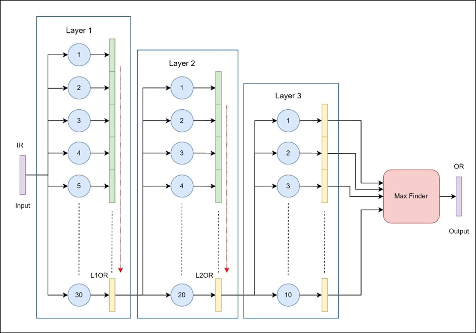
CNN Architecture and Data Flow

1. Input Data (IR):
   • The input is an 8-bit grayscale image of size 28x28 pixels.
   • It is fed to the CNN through the AXI Stream protocol, which allows for an efficient, sequential 8-bit streaming of data into the FPGA.
   • This data is fed to all neurons in Layer 1 simultaneously, allowing parallel processing at the first layer.
2. Layer 1 Processing:
   • Layer 1 contains 30 neurons (only a subset is shown in the image for simplicity).
   • The data_valid signal of the AXI stream signal is used as the input_valid signal for the layer 1 neurons.
   • Each of these neurons receives the input data, performs a weighted multiplication, adds a bias, and stores the result in a register (green) for the next stage.
   • This layer processes data in a pipelined manner, allowing all 30 neurons to compute their output concurrently. The parallelism at this stage takes advantage of the FPGA’s ability to handle multiple operations at once.
3. Data Transfer to Layer 2:
   • After Layer 1 has processed the inputs, the resulting outputs are passed to Layer 2.
   • However, due to the 8-bit transfer limitation, only the last 8 bits of each neuron’s output (highlighted in yellow) are transferred to the next layer.
   • A state machine is used for the flow control, and the contents of the large output register are shifted 8 bits at a time. The SM will drive the input_valid signal for this layer.
   • This design constraint imposes a requirement that each successive layer has fewer neurons than the previous one, so Layer 2 contains 20 neurons.
4. Layer 2 Processing:
   • Layer 2 has 20 neurons (again, only a subset is depicted in the diagram).
   • These neurons receive the 8-bit data from Layer 1, perform their own computations (weight multiplication, bias addition), and store results in another yellow register.
   • Layer 2, like Layer 1, processes data in parallel but with fewer neurons, maintaining a balanced data flow due to the pipelined design.
5. Data Transfer to Layer 3:
   • The outputs from Layer 2 are transferred to Layer 3, again restricted to 8 bits for each neuron.
   • Layer 3 contains 10 neurons, consistent with the requirement to have progressively fewer neurons in each layer.
   • This layer completes the final stage of computation, with each neuron outputting an 8-bit result.
6. Max Finder Unit:
   • The outputs of all 10 neurons in Layer 3 are fed into a Max Finder unit.
   • The Max Finder compares the output values from each neuron in the final layer and identifies the neuron with the highest activation.
   • This final output (the index of the neuron with the maximum activation) represents the network's classification decision, suitable for tasks such as identifying the digit in an MNIST dataset.

Pipelined Data Processing and Constraints

• The pipelined structure allows each layer to start processing as soon as it receives inputs, enabling overlapping computations across layers.
• Due to the 8-bit data transfer restriction, each subsequent layer has a reduced number of neurons compared to the previous one. This reduction prevents pipeline stalls and ensures a consistent flow of data between layers.

Overall Summary

1. The input data is streamed as 8-bit chunks to all neurons in Layer 1.
2. Layer 1 processes this data with its 30 neurons, and the last 8 bits of each neuron’s output are sent to Layer 2.
3. Layer 2, with 20 neurons, receives and processes the 8-bit outputs from Layer 1 and passes its 8-bit outputs to Layer 3.
4. Layer 3, with 10 neurons, produces the final neuron outputs.
5. The Max Finder identifies the neuron with the highest activation in Layer 3, producing the network’s classification output.

The neural network is clocked using the AXI clock itself, to avoid different clock domains.

Register Map

Weight and Bias load registers

Weights and Biases are loaded into the neural network using these registers.

Layer Number and Neuron Number registers

The layer number and neuron number is used to uniquely identify a neuron in the neural network, so that the respective weights and bias can be loaded into the right neuron.

Output Register

The final digit that was recognized by the network can be read from this register when the output valid bit in statReg goes high.

Status Register

0^th bit in this register indicates that the neural network has finished processing the input.

Control Register

0^th bit in this register is used to reset the whole neural network. This is also used to clear a set pending interrupt.

Training the Neural Network for Weights and Biases

Algorithms and techniques used in the training process are described below:

1. Stochastic Gradient Descent (SGD) with Mini-Batching:
   • SGD is used as the primary optimization technique, with the training data divided into mini-batches (e.g., 10 samples per batch). This allows frequent updates of weights and biases, improving training efficiency while reducing memory requirements.
2. Backpropagation:
   • The backpropagation algorithm computes the gradient of the cost function with respect to each weight and bias by propagating the error backward through the network. This is essential for calculating updates for each parameter efficiently, layer by layer.
3. Cost Functions:
   • The network supports two cost functions:
     • Quadratic Cost (Mean Squared Error), which measures the squared error between predicted and actual outputs.
     • Cross-Entropy Cost, more commonly used in classification tasks, as it penalizes incorrect confident predictions more heavily and helps avoid saturation in sigmoid-based networks.
4. Cross-Entropy Delta Calculation:
   • When using cross-entropy, the delta (error) calculation for backpropagation is optimized, resulting in faster and more stable gradient computation. This helps avoid issues like vanishing gradients that can occur with sigmoid activations in deeper networks.
5. L2 Regularization:
   • L2 regularization (controlled by a regularization parameter, e.g., lambda=5.0) discourages large weights, thereby reducing the risk of overfitting and improving generalization. This regularization term is added to the cost function, penalizing larger weights to encourage simpler models.
6. Learning Rate:
   • A learning rate (e.g., 0.1) controls the size of each step taken in the parameter space during optimization. Choosing a suitable learning rate ensures the model converges to an optimal solution without overshooting.
7. Improved Weight Initialization (Xavier Initialization):
   • The weights are initialized with a Gaussian distribution with mean 0 and standard deviation of 1number of incoming connections\frac{1}{\sqrt{\text{number of incoming connections}}}number of incoming connections​1​, a technique known as Xavier Initialization. This helps prevent vanishing/exploding gradients by keeping the magnitude of the signal consistent across layers.
8. Bias Initialization:
   • Biases are initialized using a Gaussian distribution with mean 0 and standard deviation 1, ensuring each neuron has a small initial bias value. Proper initialization helps the network learn effectively from the start.
9. Accuracy Monitoring:
   • The training process monitors accuracy on a validation set after each epoch. This helps track the network's generalization performance, allowing early detection of overfitting or underfitting.

Training Output: Weight and Bias Export

After training, the final weights and biases are exported. These pre-trained parameters can then be loaded onto FPGA with the help of MIF (Memory Initialization Files) which is supported by Vivado.

Summary

Overall, this neural network combines SGD, backpropagation, cross-entropy cost, mini-batching, regularization, and improved initialization strategies to enable efficient and stable training. These techniques make it well-suited for image classification tasks like MNIST and prepare the trained model for efficient hardware deployment.

Generating Test Data

Generating Test Data for Neural Network from MNIST Dataset

1. Loading the MNIST Dataset

The MNIST dataset is loaded from a compressed .pkl file using the load_data function. This dataset contains labeled grayscale images of handwritten digits (0 through 9) and is typically used for training and testing neural networks. The data file includes three subsets:

• Training Data: For training the network.
• Validation Data: For fine-tuning and validation during training.
• Test Data: For final model testing after training.

Each subset consists of:

• Images: Flattened arrays representing 28x28 pixel grayscale images (784 values per image).
• Labels: The corresponding digit labels (0-9).

2. Configuration for Test Data Generation

Several configuration parameters control how the test data is structured and represented in the neural network:

• Data Width (8-bits): Specifies that each test data point uses an 8-bit width, aligning with the fixed-point representation used by the neural network.
• Integer Size (1-bit): Allocates 1 bit (including the sign bit) for the integer portion, leaving 7 bits for the fractional portion. This configuration allows greater precision within the 8-bit constraint.

3. Generating Test Data Samples

The number of test data samples to generate is configurable through a command-line argument. If the argument isn’t provided, it defaults to a specific number (e.g., 3 samples).

4. Steps to Generate Test Data

Step 1: Load and Select Data

• The function retrieves the test_data subset, structured as image and label pairs, by calling load_data.

Step 2: Data Formatting

• Each test sample in test_data is an array of 784 grayscale values, with each value representing a pixel. These values are converted to the specified 8-bit signed fixed-point format, involving:
  • Scaling the Values: Adjusting the MNIST pixel values to fit the fixed-point representation.
  • Fixed-Point Conversion: Using the defined data width (8 bits) and integer size (1 bit), each value is represented with a single integer bit (including sign) and 7 fractional bits.

Step 3: Serialization and Saving

• Once formatted, the test data is serialized and saved in compressed format for efficient storage and retrieval.

5. Testing with the Neural Network

After generating the test data, it is ready to be loaded and fed into the neural network for evaluation. The test data’s fixed-point format ensures compatibility with the neural network’s input expectations, supporting consistent and accurate evaluation.

Summary of Techniques and Algorithms Used

• Data Preprocessing: Scaling and converting grayscale values to fixed-point format.
• Serialization: Utilizing serialization methods to save and retrieve test data efficiently.
• Command-Line Configuration: Allowing flexible configuration of test sample numbers through command-line arguments.

This approach ensures that the neural network receives accurately formatted test data, enabling reliable performance assessment on the MNIST dataset.

Testbench & Simulation

Testbench Architecture

Instantiations

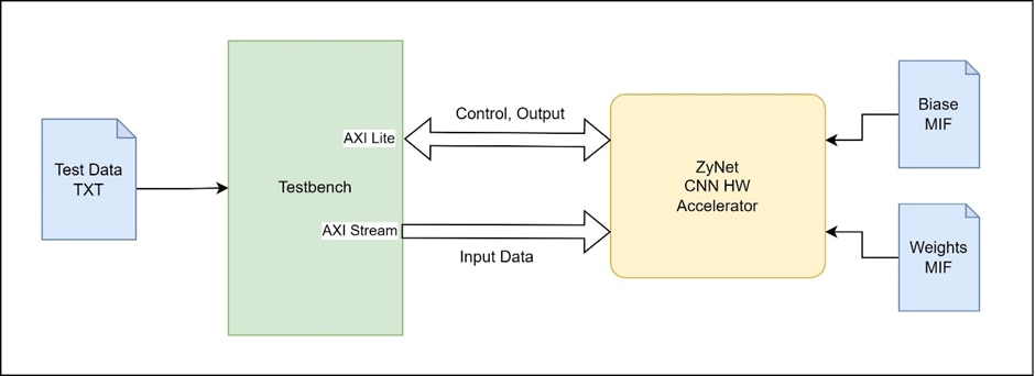
• The top module of the design which is Zynet is instantiated in the testbench. The top module has only AXI Lite and AXI Stream interfaces, hence the testbench needs to do something like a BFM to generate the required AXI signals to test the HW accelerator

Weights and Biases for the CNN

• The pre-trained weights and biases are loaded into the CNN using MIF files. These values are not changed during the test

Test Sequence

• The testbench first resets the HW
• Then it reads the test data (8-bit binary) from the TXT file and then sends it over the AXI stream interface to the Zynet module sequentially, while also handling the AXI stream control signals such as input_valid.
• It then waits for the output valid bit to get set in statReg.
• The output is then read from outputReg and compared with the expected result which is present at the end of the test data TXT file.
• The amount of data to test can be specified in the test testbench.
• The accuracy of the neural network for the number of digits tested is the ratio of correctly identified digits to the total number of digits tested.

Output

Code can be found here.

Implementation for Target: Arty Z7

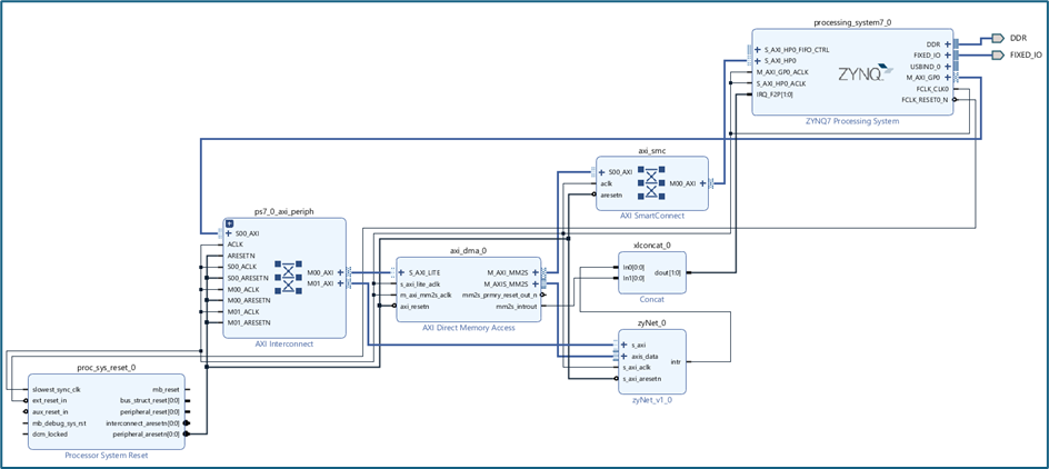
Given above is block design integrating the ZyNet in PL with the Zynq PS. The block design also contains an AXI DMA IP from AMD Xilinx for transferring the input data into the ZyNet IP.

Utilization

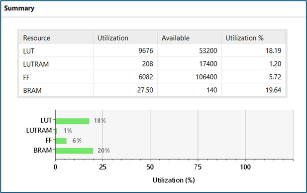
While the neuron synthesis had inferred some DSP slices, the scheduling algorithm in implementation has decided not to use them (maybe for power/performance reasons), preserving the overall functionality of the design.

On Target Testing

The hardware is exported, and the software is written with a sample Hello World template project. Test data is present in a char (8-bits) array of size (28px * 28px).

The C file flow looks something like this:

1. Initialize the AXI DMA controller
2. Initialize and connect with the interrupt controller
3. Setup and start the DMA to transfer the 768B of test data to the ZyNet module
4. Wait for the interrupt (outValid) from the ZyNet from PL fabric
5. Clear the interrupt (soft reset the ZyNet)
6. Read the output register to get the digit recognized by the ZyNet
7. Output is printed via the SDK terminal (There's a logic that checks if the pixel value is greater than 0, then print 1)

Output

C file can be found here.

Full sources used in this project can be found here.