


6.1 Instrument Interfaces
Modern bench test equipment usually support different workflows. Controlling the instrument from the front-panel has the advantage of not requiring a connected computer, but the disadvantage that the instrument's screen is small, and that the operation of the instrument may take more effort and time. Remote control of the instrument can be performed either through special programs, usually provided by the manufacturer, or through direct SCPI commands sent from custom programs.
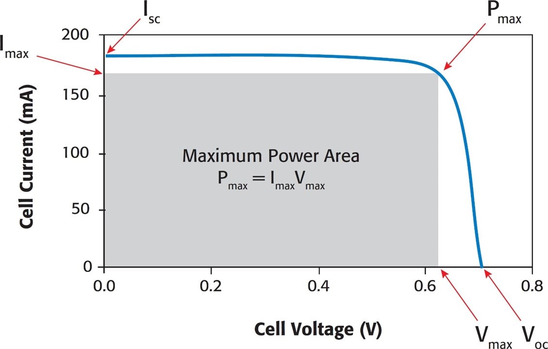
Here I will use the SMU to characterize a solar cell in terms of its short circuit current (Isc), open circuit voltage (Osc), maximum power (Pmax), and the voltage (Vmax) and current (Imax) that are required to maximize the power output using the instrument front-panel, Aim-TTi’s remote control application, and through SCPI commands sent from a Python program.
The objective is to show the different supported workflows of the instrument, and how they compare to each other. Since the focus was on the workflows, I ignored important factors that affect the I-V curve of a solar cell such as its light dependency.
For all three tests, the SMU was first set as a 0 A current source to measure the Voc, and then a sweep between 0 V and Voc was performed to find the Isc, Pmax, Vmax and Imax. The SMU was connected to the solar cell using a 2-wire connection, as illustrated in the diagram.

6.1.1 Front Panel
The “main” menu of the instrument is accessed by pressing the Cnfg button.

There are two methods to configure the instrument: Easy Setup and Manual Setup. Easy Setup allows for a quick configuration with reduced flexibility, while Manual Setup provides a broader range of setup choices at the cost of additional setup time.
In order to capture screenshots, it is necessary to press the USB icon, located in the top left corner, however, the icon is not always available. Since it is not possible to take screenshots from the Easy Setup menu, as the USB icon does not appear, I decided to use the Manual Setup, to show the available options in that menu.

I set the instrument to source current (SC Mode), use 2 wires, make continuous measurements, provide a steady output current of 0 A, automatically select the settling time, and make measurements of 1 power line cycle (PLC) of duration.
The Home button was then pressed to switch to the measurement screen, followed by a Run button press to initiate the 0 A current sourcing.

As can be seen from the image, I got a Voc of 1.631 V.
I pressed Cnfg again and set the instrument to perform a linear voltage sweep from 0 V up to 1.63 V with 164 steps. The sweep was set to be performed a single time, with a single measurement at each sweep step.

Again, Home and Run were pressed to initiate the sweep. Next, I pressed the Graph View button to plot the voltammogram (I/V curve).

The buttons in the bottom left corner, labeled as “X(+176.0 mV)” and “Y(+4.484 μA)” indicate the graticule's dimensions. However, the values selected by the instrument were not particularly useful, and despite the documentation stating that they can be adjusted, I was unable to change them to more useful values such as 200 mV/div and 5 μA/div.
To find the Isc I switched back to the home screen, pressed the “Sample Table” button and looked for the first row of the sweep table and found the Isc to be 29.11 μA.

To find the Pmax and Imax values I had to get back to the home screen, and then press Measure to change the primary and secondary measure values to current and power. This automatically changed the displayed values of the already captured table.

I then used the rotary knob to manually find Pmax, which was 17.73 μW, at an Imax of 18.27 μA. To find the Vmax, I changed the primary measurement to voltage, and found that it was 0.97 V.

Instead of searching for the values in the “Sample table”, another option is to save them to a USB drive and later analyze them in Excel, Python, Matlab, or any other suitable tool. A preview of the CSV output is provided below as an example.
Index,Step,Iteration,Date,System Time,Format,Measured time (s),Mode,M1,Units,M2,Units,M3,Units,M4,Units,CV,CC,PTol,STol
1,1,255,2023-06-27,3:3:58,24HR,0.00000e+00,SV,-1.70000e-07,Volts,-2.91169e-05,Amps,4.94987e-12,Watts,5.83853e-03,Ohms,ON,OFF,N/A,N/A,
2,1,255,2023-06-27,3:3:58,24HR,5.15137e-02,SV,1.00002e-02,Volts,-2.90603e-05,Amps,-2.90608e-07,Watts,-3.44118e+02,Ohms,ON,OFF,N/A,N/A,
3,1,255,2023-06-27,3:3:58,24HR,1.02295e-01,SV,1.99999e-02,Volts,-2.89970e-05,Amps,-5.79938e-07,Watts,-6.89724e+02,Ohms,ON,OFF,N/A,N/A,
4,1,255,2023-06-27,3:3:58,24HR,1.42578e-01,SV,3.00000e-02,Volts,-2.89403e-05,Amps,-8.68209e-07,Watts,-1.03662e+03,Ohms,ON,OFF,N/A,N/A,
5,1,255,2023-06-27,3:3:58,24HR,1.66260e-01,SV,4.00003e-02,Volts,-2.88803e-05,Amps,-1.15522e-06,Watts,-1.38504e+03,Ohms,ON,OFF,N/A,N/A,
6,1,255,2023-06-27,3:3:58,24HR,1.97021e-01,SV,5.00000e-02,Volts,-2.88240e-05,Amps,-1.44120e-06,Watts,-1.73467e+03,Ohms,ON,OFF,N/A,N/A,
7,1,255,2023-06-27,3:3:58,24HR,2.21924e-01,SV,6.00002e-02,Volts,-2.87637e-05,Amps,-1.72583e-06,Watts,-2.08597e+03,Ohms,ON,OFF,N/A,N/A,
8,1,255,2023-06-27,3:3:58,24HR,2.47803e-01,SV,7.00001e-02,Volts,-2.87009e-05,Amps,-2.00907e-06,Watts,-2.43895e+03,Ohms,ON,OFF,N/A,N/A,
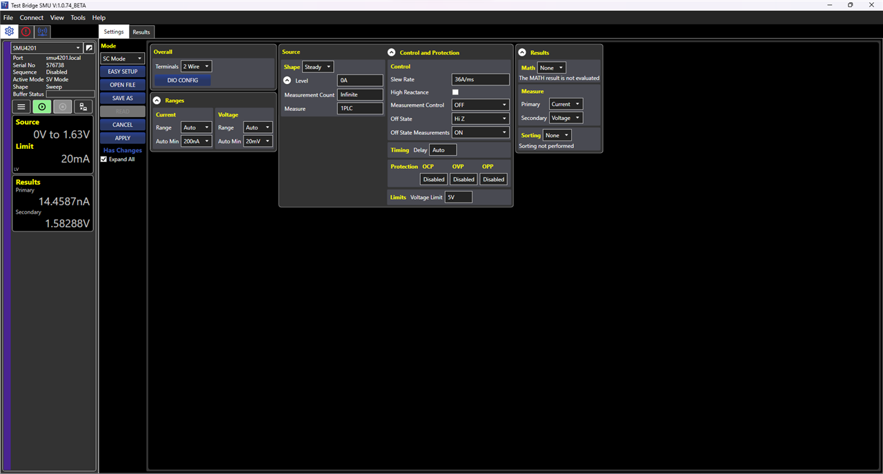
6.1.2 Test Bridge SMU
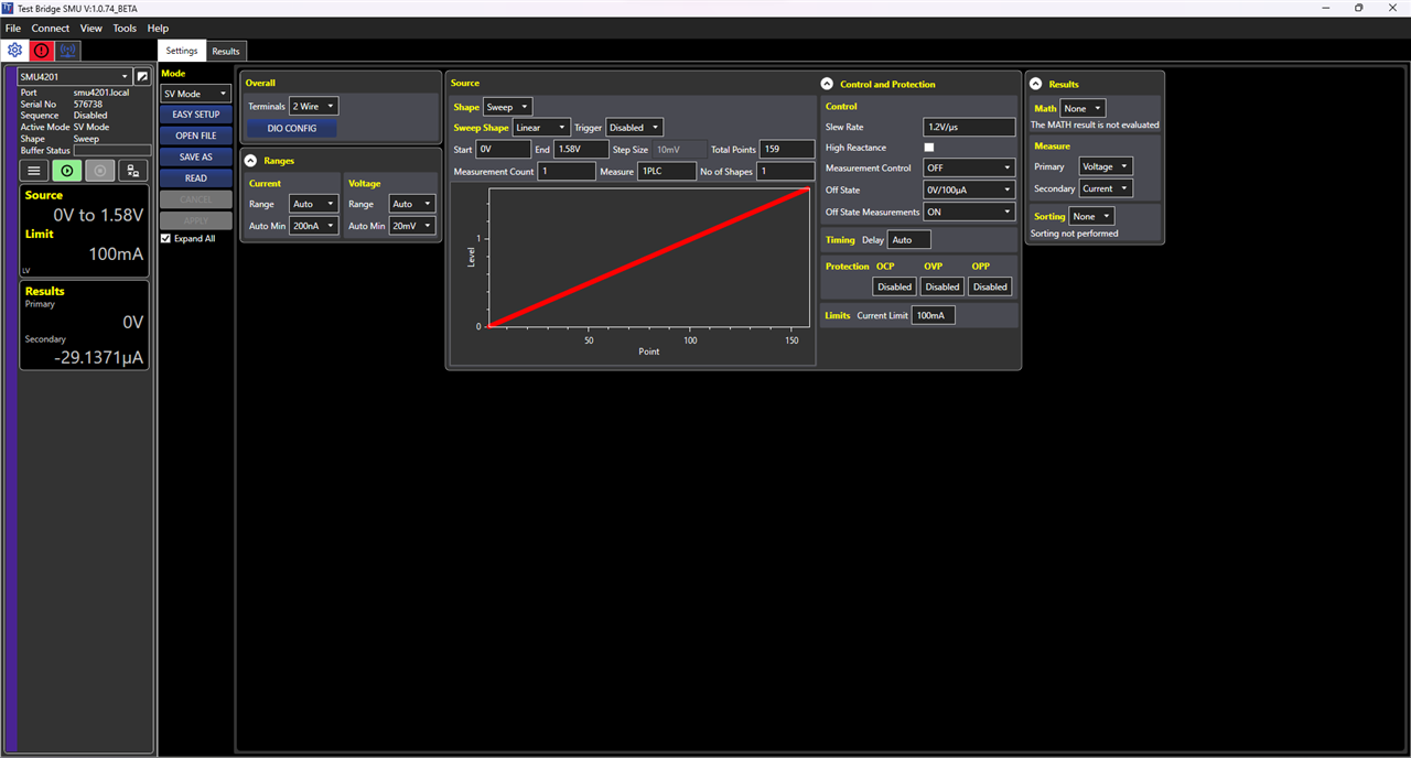
Aim-TTi's Test Bridge provides a more efficient method of programming the SMU compared to the front panel, as it provides most configuration options on a single screen.
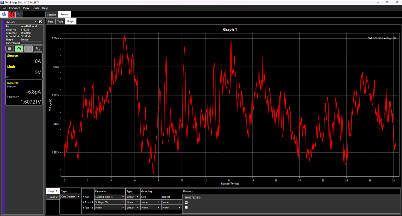
I pressed the "play" button to activate the output, and the program immediately displayed the real-time measurement of the voltage (Voc) at the left side of the screen.
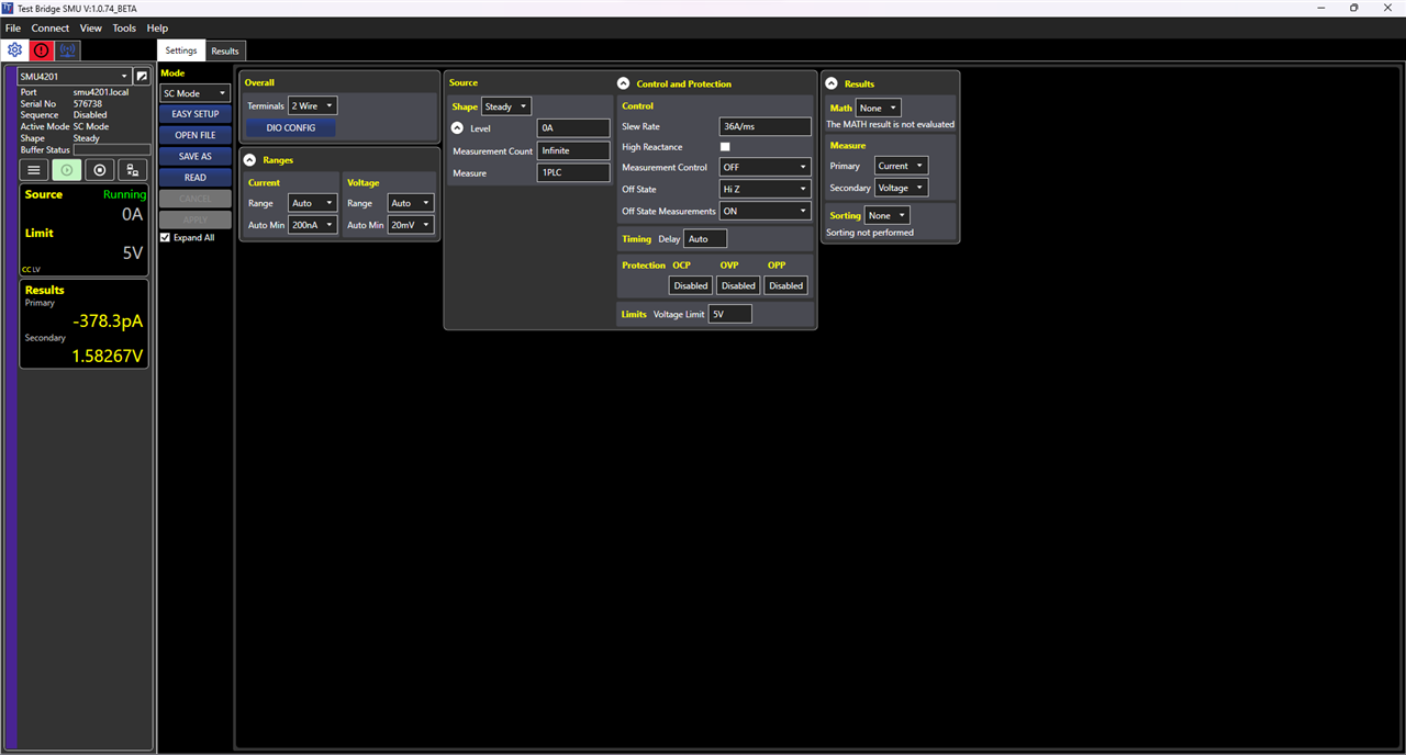
It simultaneously generated a table containing the captured data and incorporated statistical information derived from the captured data as well.
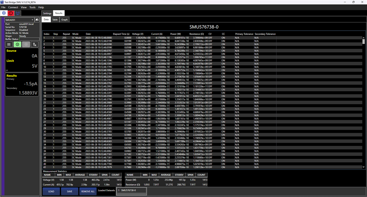
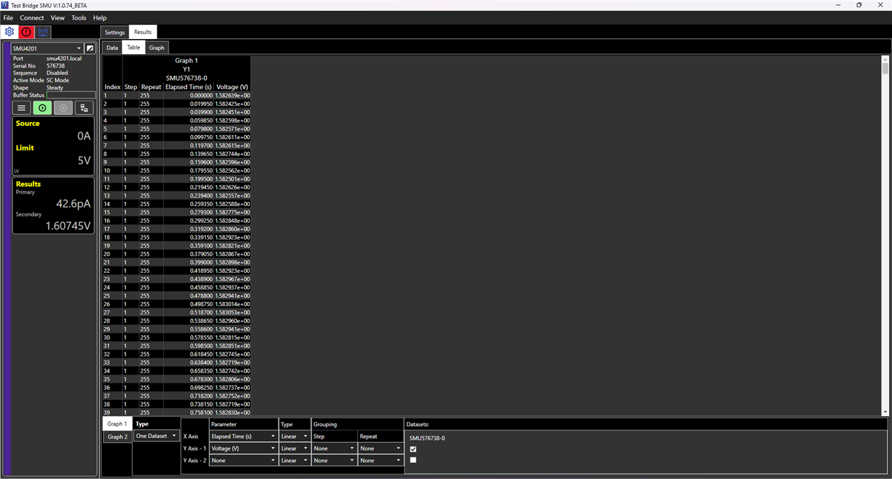
As shown in the data table, the Voc is approximately 1.583 V.
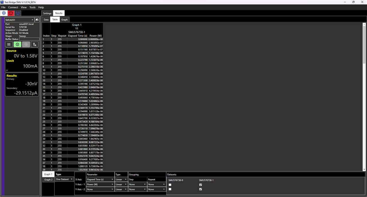
I then proceeded to select the dataset and the values to be plotted on the X and Y axes. The table used for generating the plot can be accessed in the Table tab, while the actual plot can be accessed in the Plot tab.
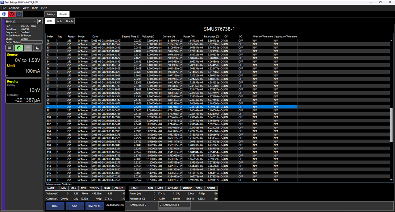
Next, I created a sweep from 0 V to 1.58 V with 159 steps.
And generated a second dataset, which I used to manually look for the Isc (29.09 μA), Pmax (17.41 μW), Vmax (0.96 V) and Imax (18.14 μA) values.
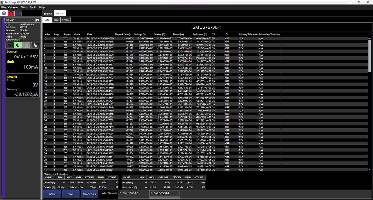
In a similar way to what I did when measuring the Voc, I generated a plot of the power curve.
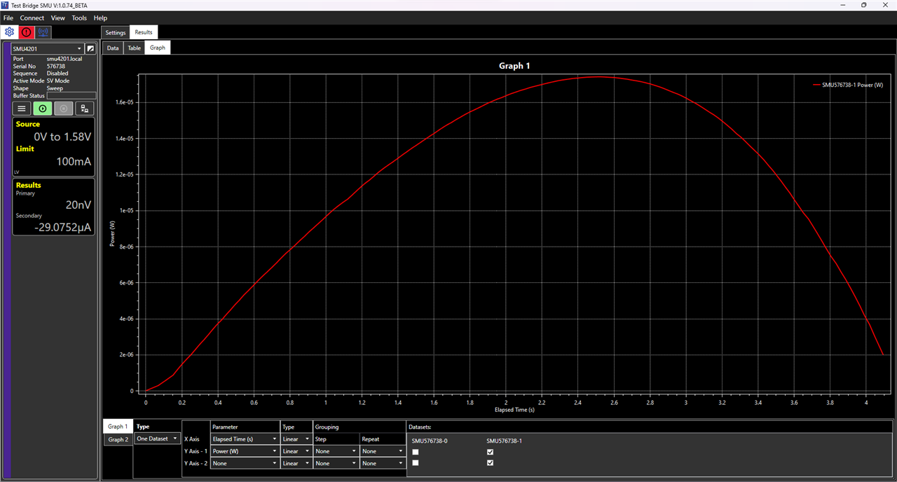
One feature that I missed in the Graph tab was the ability to track the curve to quickly get approximated Pmax, Vmax and Imax values.
As expected, it is also possible to save the dataset as a CSV file, which I found that it closely resembled the one generated by the instrument.
#
#StartTime,2023-06-28 21:05:44.0000
Index,Step,Iteration,Date,System Time,Measured time (s),Mode,M1,Units,M2,Units,M3,Units,M4,Units,CV,CC,PTol,STol
1,1,255,2023-06-28,21:05:44.0000,0,SV Mode,-0,Volts,-2.909239992732182E-05,Amps,0,Watts,0,Ohms,ON,OFF,N/A,N/A
2,1,255,2023-06-28,21:05:44.0688,0.06885999999940395,SV Mode,0.010000109672546387,Volts,-2.9038599677733146E-05,Amps,2.903891815145016E-07,Watts,344.3729995084608,Ohms,ON,OFF,N/A,N/A
3,1,255,2023-06-28,21:05:44.1109,0.11095000000022992,SV Mode,0.020000120624899864,Volts,-2.8975300665479153E-05,Amps,5.795095084523244E-07,Watts,690.2472162688473,Ohms,ON,OFF,N/A,N/A
4,1,255,2023-06-28,21:05:44.1511,0.15115999999943597,SV Mode,0.029999900609254837,Volts,-2.8916800147271715E-05,Amps,8.675011303558371E-07,Watts,1037.4557508599482,Ohms,ON,OFF,N/A,N/A
5,1,255,2023-06-28,21:05:44.1740,0.17406999999911932,SV Mode,0.04000059887766838,Volts,-2.8853799449279904E-05,Amps,1.1541692578673343E-06,Watts,1386.319987008389,Ohms,ON,OFF,N/A,N/A
6,1,255,2023-06-28,21:05:44.1979,0.19794999999976426,SV Mode,0.05000019818544388,Volts,-2.8793399906135164E-05,Amps,1.4396757017394994E-06,Watts,1736.5159497816048,Ohms,ON,OFF,N/A,N/A
7,1,255,2023-06-28,21:05:44.2237,0.22379000000000815,SV Mode,0.06000009924173355,Volts,-2.8731199563480914E-05,Amps,1.7238748251429065E-06,Watts,2088.325588674595,Ohms,ON,OFF,N/A,N/A
8,1,255,2023-06-28,21:05:44.2513,0.2513600000002043,SV Mode,0.06999970227479935,Volts,-2.866870090656448E-05,Amps,2.006800528064784E-06,Watts,2441.6768134328336,Ohms,ON,OFF,N/A,N/A
9,1,255,2023-06-28,21:05:44.2751,0.27511000000049535,SV Mode,0.08000019937753677,Volts,-2.860389940906316E-05,Amps,2.288317655700059E-06,Watts,2796.82844053733,Ohms,ON,OFF,N/A,N/A
10,1,255,2023-06-28,21:05:44.2988,0.2988900000000285,SV Mode,0.09000039845705032,Volts,-2.8540300263557583E-05,Amps,2.568638395804041E-06,Watts,3153.449600247186,Ohms,ON,OFF,N/A,N/A
6.1.3 SCPI
To programmatically control the instrument and find the solar panel parameters I wrote a Python program. The SCPI programming interface is straightforward, but the brief SCPI documentation with few usage examples, added difficulty to the task of properly controlling the SMU.
To measure the solar panel parameters, I wrote the following program:
import numpy
import csv
import time
import pyvisa


# write an SCPI command and wait for the instrument to process it
def write(command):
    smu.write(command)
    smu.query('*OPC?')

# Make an SCPI query
def query(command):
    response = smu.query(command)
    return response

# Wait for the instrument to complete the sourcing task
def wait():
    while True:
        condition = int(query('STATus:OPERation:CONDition?'))

        if condition & 0x1000 != 0:
            break

        time.sleep(0.01)

# Read the instrument measuring buffer and return its contents a 3 column (primary measurement, secondary measurement, time) matrix.
def read_data():
    string = query('MEMory:DATA:BUFFer:ASCii?')
    string_list = list(csv.reader([string]))[0]
    float_array = numpy.array([float(x) for x in string_list]).reshape((-1, 3))
    return float_array


# Connect to the instrument's raw TCP server
smu = pyvisa.ResourceManager().open_resource('TCPIP::192.168.0.33::5025::SOCKET')
smu.read_termination = '\n'
smu.write_termination = '\n'

write('*RST')                                               # Reset the SMU (i.e: Set the parameters to their default state)

write('SYSTem:FUNCtion:MODE SOURCECURRent')                 # Set the SMU as as a current source
write('SOURce:CURRent:MEASure:PRIMary VOLTage')             # Set primary measurement variable to voltage
write('SOURce:CURRent:MEASure:SECondary CURRent')           # Set secondary measurement variable to current
write('SOURce:CURRent:SHAPe FIXed')                         # Set output to a fixed current
write('SOURce:CURRent:MEASure:COUNt 1')                     # Make a single measurement
write('SOURce:CURRent:FIXed:LEVel 0')                       # Set current output to 0 A
write('OUTPut:STATe ON')                                    # Begin sourcing 0 A, make 1 I-V measurement and then turn off the output
wait()                                                      # Wait for the SMU to finish
data = read_data()                                          # Read the I-V values

voc = data[0, 0]                                            # Store the Voc value

steps = int(voc * 100) + 1                                  # Calculate the number of steps required to increase the voltage 10 mV at every step of the voltage sweep
max_v = float(int(voc * 100)) / 100                         # Set the maximum voltage of the sweep

write('SYSTem:FUNCtion:MODE SOURCEVOLTage')                 # Set the SMU as voltage source
write('SOURce:VOLTage:MEASure:PRIMary VOLTage')             # Set primary measurement variable to voltage
write('SOURce:VOLTage:MEASure:SECondary CURRent')           # Set secondary measurement variable to current
write('SOURce:VOLTage:SHAPe SWEep')                         # set the output as a voltage sweep
write('SOURce:VOLTage:SHAPe:COUNt 1')                       # Perform a single sweep
write('SOURce:VOLTage:MEASure:COUNt 1')                     # Perform a single measurement at each sweep step
write('SOURce:VOLTage:SWEep:SPACing LINear')                # Perform a linear voltage sweep
write('SOURce:VOLTage:SWEep:POINts {:d}'.format(steps))     # Set the number of voltage sweep steps
write('SOURce:VOLTage:SWEep:STARt 0')                       # Set the initial value to 0 V
write('SOURce:VOLTage:SWEep:STOP {:f}'.format(max_v))       # Set the last value of the voltage sweep to max_v
write('OUTPut:STATe ON')                                    # Initiate the swwep, make the I-V measurements and then turn off the output
wait()                                                      # Wait for the SMU to finish
data = read_data()                                          # Read the I-V values

isc = -data[0, 1]                                           # Store the Isc value

power = -data[:, 0] * data[:, 1]                            # Compute power
index = numpy.argmax(power)                                 # Find the array index with the maximum power value

pmax = power[index]                                         # Store Pmax
vmax = data[index, 0]                                       # Store Vmax
imax = -data[index, 1]                                      # Store Imax

# Print the values
print('Voc  = {:7.3f} V'.format(voc))
print('Isc  = {:7.3f} uA'.format(isc * 1E6))
print('Vmax = {:7.3f} V'.format(vmax))
print('Imax = {:7.3f} uA'.format(imax * 1E6))
print('Pmax = {:7.3f} uW'.format(pmax * 1E6))

smu.close()
Which generated the following output:
Voc  =   3.549 V
Isc  = 236.154 uA
Vmax =   2.310 V
Imax = 168.920 uA
Pmax = 390.204 uW
6.1.4 Conclusions
As expected from a reputable test equipment company, the SMU supports different workflows to suit diverse needs. The front panel-interface is highly intuitive and user-friendly, with the drawback that requires time to set all the parameters. The Test Bridge SMU application on the other side, provides the convenience of viewing and setting all parameters on a single screen. It offers better plotting capabilities compared to the SMU's small screen and, as of now, is available for free. While the application has some bugs, they are not critical enough to render it unusable. On the other hand, SCPI commands are especially valuable for automation purposes and when working with complex protocols, as they provide the greatest flexibility to control the instrument. Nevertheless, I found two areas of the SCPI subsystem that could be improved: its stability (during development, I had a few freezes) and the inclusion of support for other interfaces such as VX11 or HiSLIP, which offer some advantages over raw TCP.