


Overview
In my previous part 1 and part 2 posts I showed how I started to work on this roadtest, how I setup an RF communication link on the Texas Instruments Value Line Development Kit CC11XLDK-868-915, and how I started to measure various characteristics of the transmitter using the Agilent/Keysight N9322C spectrum analyzer. In this post I will continue with the characterization of the transmitter and the communication link.
More Analysis of GFSK Demodulated Data Packets
I first setup a communication link between one SmartRF board with CC115L transmitter module and one SmartRF board with CC113L receiver of the TI CC11XLDK-868-915 kit. In the SmartRF Studio control panel I selected GFSK modulation format, packet data size 30 (28+2), and packet count infinite. Next I connected the Diamond RH799 wide bandwidth antenna to the N9322C spectrum analyzer and I looked at the demodulated signal. The modulation analysis function built in the spectrum analyzer can display the demodulated waveform in time domain, in eye-diagram format, and also in demodulated packet data symbols. The picture below shows the demodulated waveform:
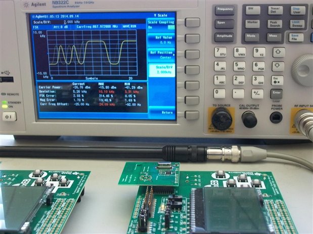
We can see in this picture the pulses corresponding to logic “1” and logic “0” symbols. They are shifted either down to –5.157kHz level on y-axis or up to +5.157kHz level. The same data can be represented in eye-diagram format, as I am showing in the picture below:
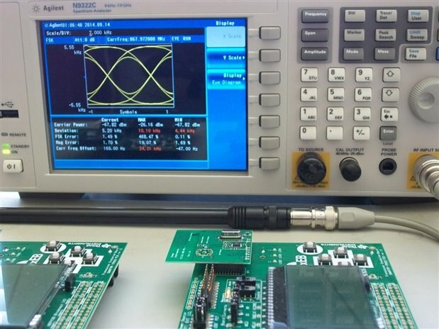
What bothered me was the fact that I saw demodulation errors reported at the bottom of the screen, like FSK Error and Mag Error. I decided to spend some time trying to understand why these errors are reported there. On the SmartRF Studio control panel all the packets were received correctly without any error. I tried to adjust the settings of the spectrum analyzer demodulation parameters, but I couldn’t make the errors disappear. However, from all these tries I noticed that the demodulated waveform sometimes stops or has glitches, and I assume that the transmitter does not send data continuously, which may “trick” the demodulator inside the N9322C spectrum analyzer. But why the SmartRF Studio showed that all packets have been received correctly without errors? My assumed explanation for this is that SmartRF Studio controls both transmitter and receiver boards, and knows when a packet is transmitted and when it stopped or when there are preambles or transitions that create demodulated glitches. Knowing this information SmartRF Studio may process only the valid packets and may ignore all the transient stop/start/glitches when checking for errors.
To further understand if my assumption is correct I setup the N9322C spectrum analyzer to display the demodulated packet data. This is a nice feature of the built-in modulation analysis function. So what I noticed was that when I looked at multiple data packets the symbol values were wrong, either all “1” or all “0”; however, if I looked at only one data packet at a time the bits were correct. The following picture shows one demodulated data packet of 30 symbols displayed by the N9322C spectrum analyzer.
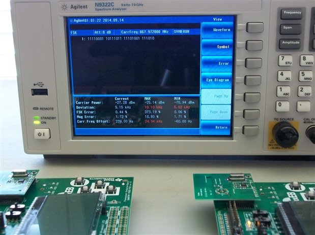
I think this may happen because of the stop/start/glitches that I saw in the waveform between data packets, which may be taken care of in SmartRF Studio since it knows when the transmitter sends valid data, but not in the spectrum analyzer which does not know what the transmitter is controlled to do at each moment in time.
N9322C Reflection Measurement Calibration
In this experiment I mounted an SMA connector on one of the CC110L transceiver module and I connected an external antenna using three combinations of different RG58 cable lengths. The purpose was to check the effects of the cables and connectors on the frequency spectrum measured with Agilent/Keysight N9322C spectrum analyzer and the degradation of bit error rate (BER).
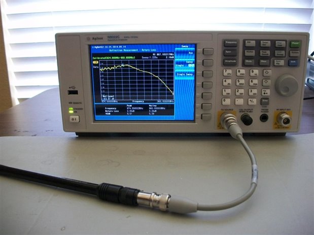
But first I wanted to measure the losses of these three cables, so I used the built-in tracking generator and reflection measurement function of the Agilent/Keysight N9322C spectrum analyzer. I turned on the spectrum analyzer and I set it in the reflection measurement operation mode. Then I selected the frequency range for these measurements around the carrier frequency of the transmitter, from 824MHz to 960MHz (the carrier frequency was 867MHz). Then I looked at the next screen, shown in the picture below, and I noticed the word “Uncalibrated” displayed in the upper left corner, which basically told me that I need to perform a calibration procedure before measuring the cable loss.
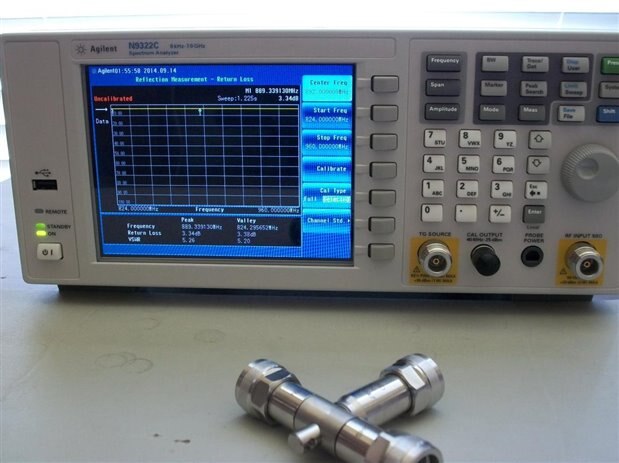
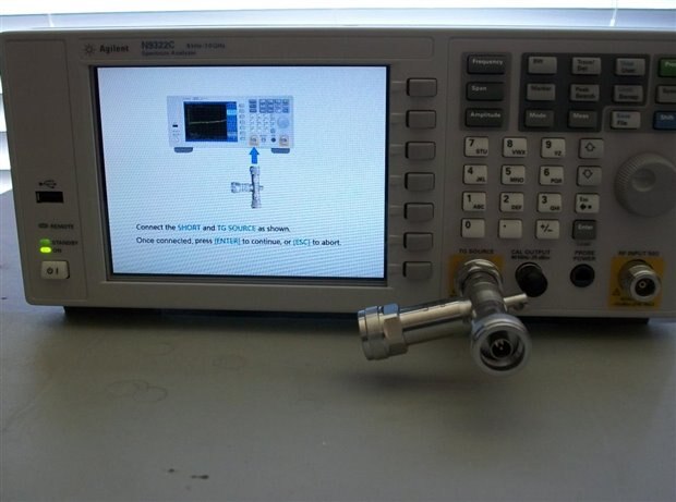
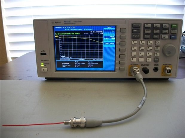
The N9322C spectrum analyzer was shipped with a calibration “T” shown in the picture above. This calibration device has three ports with three different input impedances. One port has infinite impedance “open”, another port has zero Ohm impedance “short”, and the other port has 50 Ohms impedance "load". So I started the calibration process by pressing the “Calibrate” button on the N9322C side buttons. Then I really liked how the N9322C spectrum analyzer guided me through the entire calibration procedure. First N9322C prompted me (and also showed me how to) connect the calibration device “open” port to the TG source output, as I am showing in the following picture.

Next I pressed “Enter” and the spectrum analyzer performed the calibration step in about 1-2 seconds. Then it prompted me to connect the calibration device “short” port.
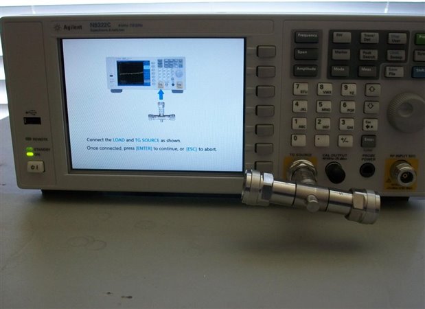
I connected it and then I pressed “Enter” and the spectrum analyzer performed the “short” calibration step. After that it prompted me to connect the 50Ohms load port of the calibration device.
After this calibration step the spectrum analyzer went back to the reflection measurement screen, but this time it displayed “Calibrated” in the upper left corner and it also displayed the calibration frequency range.
Measurement of Return Loss of Cables and Antennas
I used three cables: cable1 was a single piece about 3ft long of RG58 coaxial cable, cable 2 was made out of two cable1 pieces connected with a coaxial adapter, and cable 3 was made out of three pieces of the same type of cables connected together. Besides these cables I also wanted to measure the return loss of the Diamond RH799 wideband antenna that came with the spectrum analyzer and another “home-made” antenna that I am showing in the figure below.
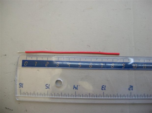
This antenna is made out of a simple wire sized at lambda/4 of the TX carrier frequency.
The cable loss measurements are shown in the following pictures.

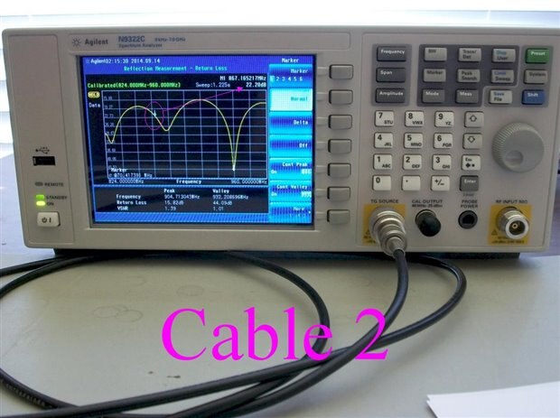
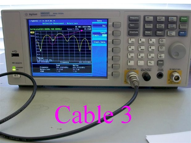
In these measurements I used the marker function of N9322C to measure the return loss at the TX carrier frequency, as I have annotated in the figures above. Notice also more resonant peaks for cables 2 and 3 compared to cable 1. These additional resonance peaks are due the mismatch in characteristic impedance of coaxial adapters used to connect the individual cables together.
The following two pictures show the return loss measurements for the two antennas that I mentioned above, the wideband (Diamond RH799) and my home-made wire antenna.
Of course as I expected the Diamond RH799 performs better, but mine looked good too.
Measurement of VSWR
The Agilent/Keysight N9322C spectrum analyzer can also measure one-port insertion loss and voltage standing wave ratio (VSWR). VSWR is a parameter that measures how well the cable + antenna characteristic impedance is matched to the expected 50 Ohms of the transmitter output impedance. An ideal impedance match produces a VSWR = 1 and in non-ideal cases VSWR has values larger than 1. So first I measured the VSWR of the 50 Ohms load as I am showing in the picture below.
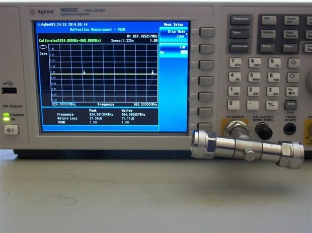
The measurement window shows the peak and valley values of the VSWR over the measurement frequency range, and we can see that both reported VSWR values equal to 1. Next I measured the VSWR of each of the three cables, and the results are shown in the pictures below.
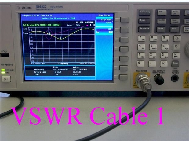
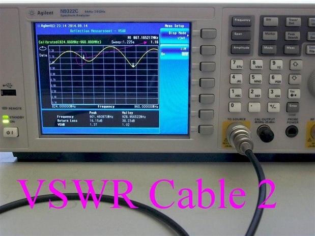
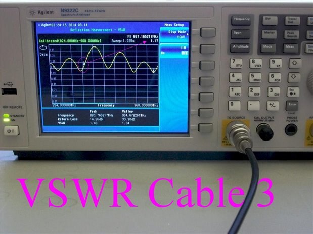
From the measurement window at the bottom of the screen we can see that cable 1 has VSWR values between 1.05 and 1.34, cable 2 has VSWR between 1.02 and 1.37, and cable 3 has VSWR between 1.04 and 1.48. So the minimum values don’t vary significantly among these three cables, but the maximum values increase sequentially: 1.34, 1.37, 1.48. As shown annotated on the pictures, for each cable I used the built-in marker to measure the VSWR at the carrier frequency of 867MHz. The VSWR values at carrier frequency do not vary significantly among the three cables.
Transmitter with External Antenna
In the next experiment I connected my home-made antenna to the CC110L transceiver in four setups: first directly without any cable, second through cable 1, third through cable 2, and fourth through cable 3. In each case I used the SmartRF Studio software to setup a communication link that transmitted continuously data packets in FSK modulation mode, and I studied the effect of cables loss on the signal received by CC113L and on the reported bit error rate (BER).
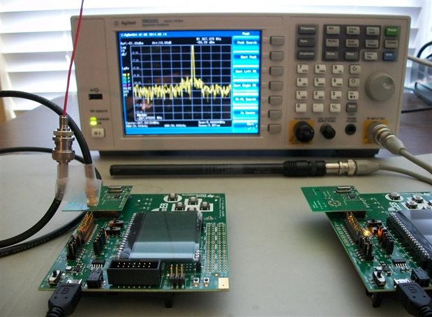
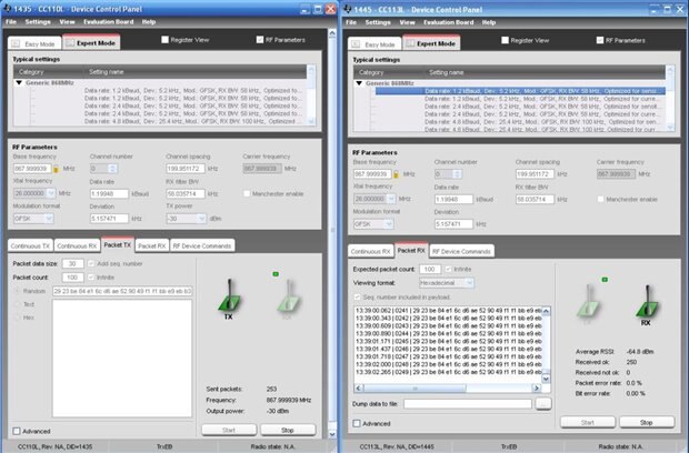
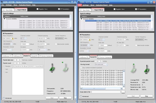
First I connected my home-made antenna directly to the CC110L transceiver SMA connector. Here is a picture of the measurement setup followed by a screenshot of the SmartRF Studio control panels.
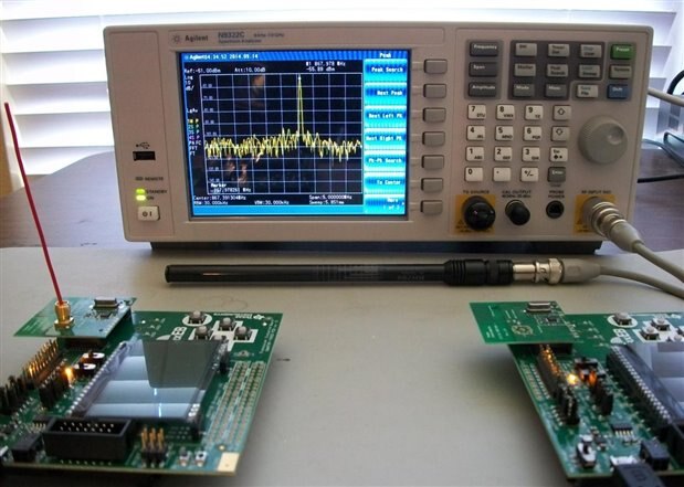
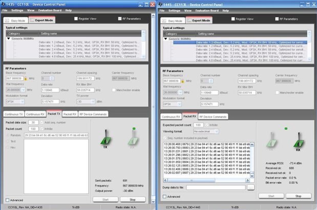
So the average Return Signal Strength Indication (RSSI) at the receiver is –73.4dBm and there are no bit error rate (BER) errors; all data packets are received correctly.
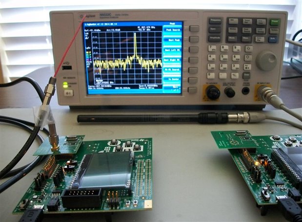
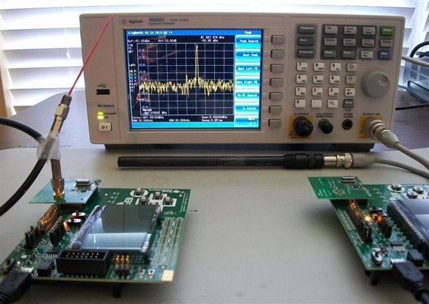
Next I connected my home-made antenna through cable 1. The picture below shows the experiment setup and N9322C measured spectrum followed by a screenshot of the SmartRF Studio control panels.
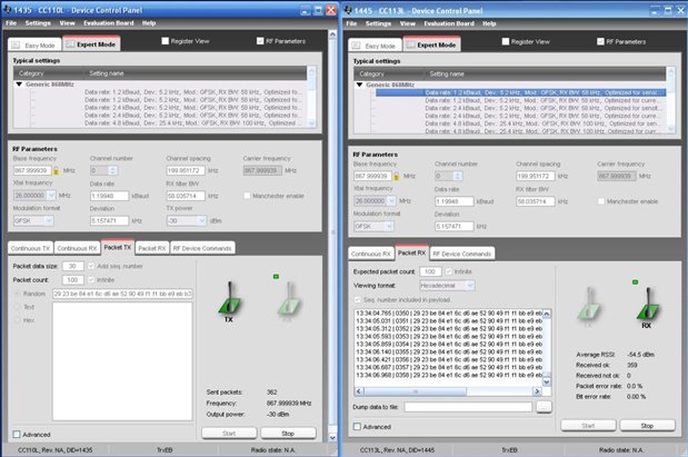
The average RSSI at the receiver is –54.5dBm, which surprisingly came higher than the antenna only case above. I suspect there might be some resonance created by the combination of SMA mounting parasitics and mismatch into antenna when I connect the antenna directly without cable. Before thinking more about this discrepancy I wanted to see what happens with the other two cables. The picture below shows the experiment setup of the antenna connected through cable 2 followed by a screenshot of the SmartRF Studio control panels.
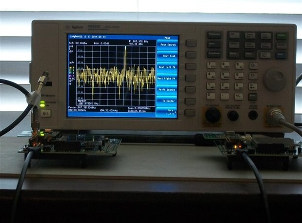
The average RSSI dropped to –64.8dBm, which makes sense since I expect cable 2 to introduce more reflection losses than cable 1. Next I inserted cable 3. The following picture shows the setup and N9322C measured spectrum followed by a screenshot of SmartRF Studio control panels.
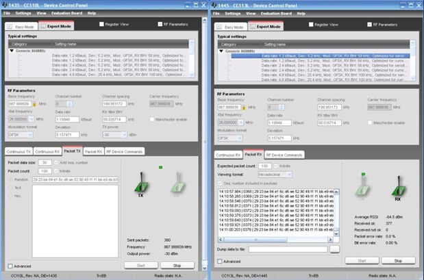
The average RSSI is –64.4dBm, almost at the same value as for cable 2. I expected cable 3 to introduce more losses than cable 2 but it did not happen. My only explanation is that there are multiple factors involved here and very possibly not the length of the cable is the dominant factor but the impedance discontinuity of connectors on the cable. Cable 1, which is just one piece, shows lower losses that cables 2 and 3, which are made out of multiple pieces connected together with coaxial adapters.
In addition to checking the average RSSI level I also checked the BER (bit error rate), and in all cases the BER was zero, which means that all the data packets came to the receiver without any error. Further more, I wanted to see if I could make BER to show errors, so I removed the antenna completely from the transmitter. The picture below shows this experiment and it is followed by a screenshot of SmartRF control panels.
The RSSI level dropped to –93.6dBm and I waited until 2200 data packets have been sent, but BER was still zero. So I couldn’t make BER fail even after I removed the antenna from the transmitter. My explanation is that the TX and RX SmartRF boards were quite close to each other on the test bench and the radiation level was enough to transmit a signal to the receiver. The receiver may also have a high sensitivity contributing to this. I expect that if I move the receiver in a different room I would be able to make the BER fail.
Distance to Fault Measurement
A nice feature built in the Agilent/Keysight N9322C spectrum analyzer is the distance to fault measurement, which basically measures the distance to characteristic impedance discontinuities along the transmission line cable (typically coaxial type but it should work with PCB traces and basically any type of transmission line). This is a great feature of N9322C since typically these types of measurements are done with Time Domain Reflectometry (TDR) functions of expensive oscilloscopes. The physical principle is to send a signal through the measured cable and analyze the time that it takes to receive back reflected parts of that signal. Based on this time and the velocity of signal through the cable the instrument can calculate the distance to the impedance discontinuity that generated the partial reflection. My next experiment uses the distance to fault feature of the Agilent/Keysight N9322C spectrum analyzer to measure a "compound" cable made of the short gray cable that came with the spectrum analyzer and two 3ft long RG58 cables connected together. But first I needed to recalibrate the spectrum analyzer for a wider range of frequencies, 5MHz to 7GHz, following the same procedure as for the reflections measurements. Next I connected the "compound" cable to the TG Source connector on the front panel of N9322C, and I selected the distance-to-fault measurement mode. Here is a picture of this experiment setup with my annotations in pink.
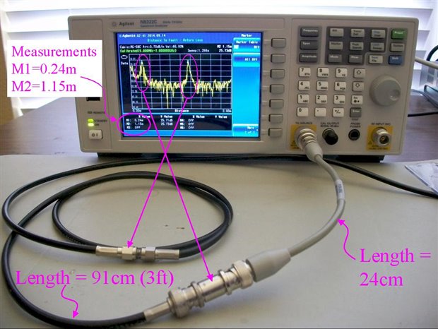
So my cable was made out of three segments: first the short cable that came with the spectrum analyzer and which measures about 24cm, second a piece of RG58 cable of 3 feet length (about 91cm), and the third another piece of RG58 cable. These cables have around 50Ohms characteristic impedance, but the adapters that connect them together introduce impedance discontinuities. These impedance discontinuities generate partial reflections as the signal travels through the cables. The partially reflected signals travel back to the spectrum analyzer, which computes the distance to the reflection point. If we look at the trace on N9322C screen starting from the left we see two spikes that I have encircled with pink color. The first spike represents the reflection from the first interconnect on the cable and the second spike represents the reflection from the second interconnect, as I have annotated with the two pink arrows. To measure the distance I then used the marker feature of the N9322C spectrum analyzer, and I placed one marker on the first spike and another marker on the second spike. Then at the bottom of the screen I could read the distance to first marker as 0.24m and the distance to the second marker as 1.15m. The picture below shows a magnified view of the N9322C screen.
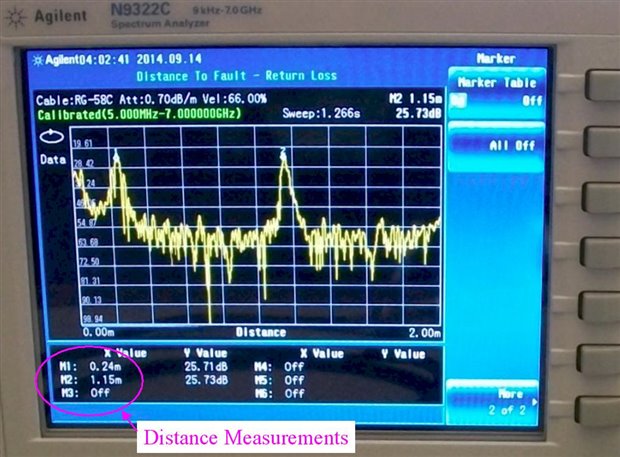
The first measurement of 0.24m matches the length of the short gray cable of 24cm. The second measurement of 1.15m matches the sum of the lengths of the short cable and one piece of RG58 cable: 91cm + 24cm = 115cm. This was just an experiment where I knew the location of the impedance discontinuities, and the measurement results proved that the distance-to-fault measurement using N9322C can be used to determine the locations of the impedance discontinuities. The distance-to-fault function of N9322C becomes very useful in the design and troubleshooting of transmission lines since it can detect otherwise hard to find impedance discontinuities issues.
This concludes the third set of measurements that I have done with the Agilent N9322C spectrum analyzer on the Texas Instruments CC11XLDK-868-915 development kit. I have a few more experiments on my list and I will include them in the roadtest review next week.
Best Wishes,
Cosmin


