


Introduction
In an earlier blog post, the use of a Vector Network Analyzer was introduced for the general reader. Continuing the simple no-maths approach, this short blog post walks one through how to use the VNA to perform an easy but exciting exercise; measuring an inductor!
I’ll be using the FPC1500 VNA, but the information here is relevant to all VNAs; nothing device-specific will be performed.
Calibrating the VNA for Measurements
First, switch on the VNA, let it warm up for at least a few minutes (ideally longer!), and connect a cable to it. This example uses an SMA cable with an SMA male connector at the device-under-test end.
Recalling the earlier blog post, the VNA needs to be made aware of where the end of your cable is because it will measure reflected signals to determine impedance, so the location of reflection needs to be known by the VNA, and it can achieve that, using a procedure known as Open/Short/Load (OSL) calibration.
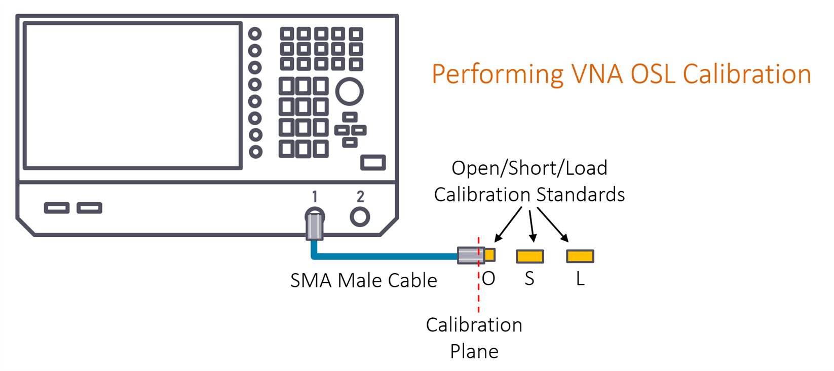
As discussed in that earlier blog post, when you perform a calibration using OSL standards, the calibration will occur at a particular reference position or plane, which is set by the connector standard drawings, and the OSL coefficients that were configured into the SMA. The earlier discussion shows how to build DIY OSL standards and how to approximately arrive at the coefficients (if, however, you purchase ready-made OSL standards, then they will come with the coefficients, all ready for entering them into the VNA).
Whichever VNA model you’re using, there will be a menu of some sort that will allow you to enter those coefficients.
Follow the VNA prompts and perform the OSL calibration using the Open, Short, and Load standards. The VNA will tell you when to attach them, so you simply need to follow what it says on its screen!

You now have a VNA calibrated and ready for measurements at the reference plane.
However, your device-under-test will not be soldered at that calibration reference plane because that’s a few millimeters inside the SMA connector! The next step will, therefore, be to attach a short extension, i.e. whatever is needed to eventually solder your device-under-test (DUT).
Physically Moving the Reference Plane
In the inset photo below, you can see that a bare SMA female connector has been attached to the male SMA connector. The bare connector is an open circuit. Notice that the Smith chart does not indicate a single dot at the far right side (remember, the horizontal line indicates pure resistance, and the far left size is zero ohms, and the right side is infinite resistance, i.e., an open circuit); instead, it is a line going southward; you’re seeing capacitive reactance. That’s because, from the reference plane point of view, you’ve attached two conductors (the center and outer parts of the female SMA connector), and two conductors separated by an insulator form a capacitance.

Side note: As you approach microwave frequencies and beyond, the length of the SMA legs and the wires to the inductor will cause more significant measurement error, and other approaches will be required, such as using a different test fixture (this may be covered in a future blog), and performing de-embedding (which was discussed in the first blog).
At this point, you can either get your VNA to perform electrical length compensation automatically, or you can capture a Touchstone file (which contains the trace data) for later calculation with Python code.
Not all VNAs may support electrical length compensation, therefore we will proceed with the Python method, so in the VNA menu, select the option to save the S11 data to a .s1p format file. Call it something like test-open.s1p.
Measuring the Device-Under-Test (DUT)
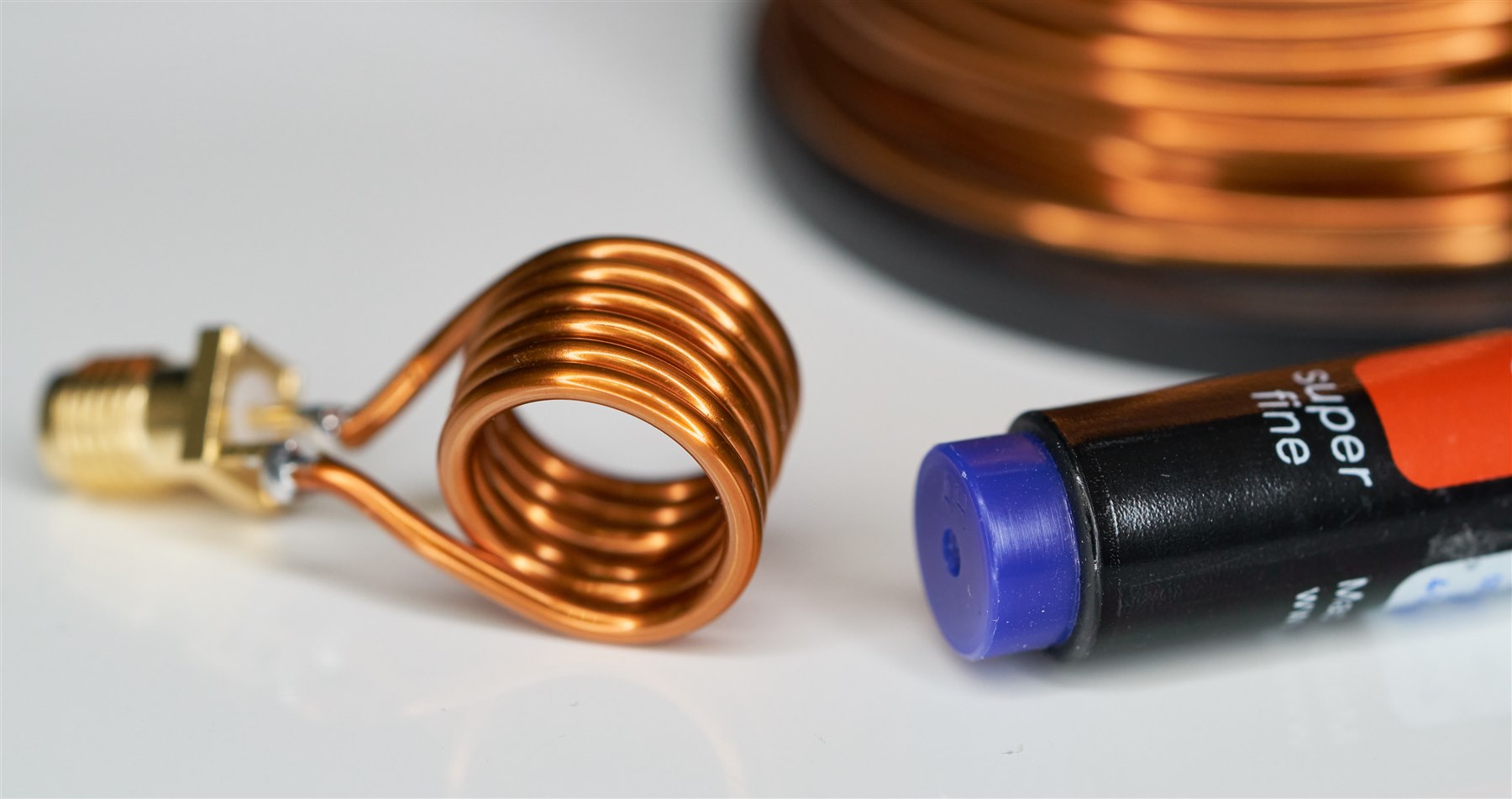
Now, solder the inductor to the connector and re-attach it to the VNA. The result is shown in the screenshot below. Notice (by looking at the marker position M3) that in this example, the trace reaches the horizon at about 250 MHz, and beyond that, the coil of wire looks capacitive. That’s normal because a coil of wire is really an inductor with a small capacitance in parallel, i.e., it is an LC circuit, and beyond some frequency (250 MHz in this case), the combined LC circuit has capacitive reactance.
None of the measurements (particularly those at high frequency) are of any use currently though, because the VNA is looking at things from the calibration reference plane, whereas we only want to look at the coil of wire.

As before, select the option to save the measurements in the VNA menu. This time, call the file something like test-inductor.s1p.
Now you have two .s1p files, and using those, a corrected output can be computed.
Electrical Length Compensation
From the previous two steps, we now have inductor measurement plus the measurement of an open circuit at the location where the inductor was soldered. These measurements are in the form of .s1p files. Now the two files will be converted into a single corrected file. Edit the elec_comp.py program that was discussed earlier, as follows:
open_fname = 'test-open.s1p'dut_fname = 'test-inductor.s1p'
Run the program as described earlier:
pip install scikit-rfpip install matplotlibpip install scypipip install numpypython ./elec_comp.py
A chart will be displayed on the screen, and a new file called corrected.s1p will be created!
Plotting the Result
You can now use whichever software you like to examine the corrected.s1p file, or you can open it in Notepad. As another option, I wrote a short plot_ind.py Python program to chart the inductance versus frequency. Edit the line in the Python code to set the filename:
dut_fname = 'corrected.s1p'
When run (type python ./plot_ind.py) it will read the corrected.s1p file, and display a chart. You can drag the red marker to the desired location of interest. A zoom button is available in the icons at the bottom of the chart.
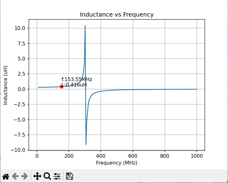
From that chart, it can be seen that the inductance at about 150 MHz is 416 nH, and that the resonant frequency is about 300 MHz.
As a sanity check, any free online air-core coil calculator could be used to see if the inductance is right. In my case, I had six turns, with approximately 13 mm diameter and a length of about 9mm. Online calculators will indicate a value of around 403 nH, so this provides a lot of confidence in the measurement!
Summary
The VNA can provide immense detail into inductor measurements (and any passive network measurements). The procedure first involves calibrating the VNA using OSL standards and then attaching your fixture where the DUT (the inductor in this example) will be soldered.
Two measurements are needed, with and without the DUT, so that an Electrical Length Compensation can be carried out (either using the VNA’s built-in capabilities or, alternatively, using Python code on a PC).
The blog post discussed how to capture the measurements into Touchstone format .s1p files, and then Python code was used to generate a corrected output .s1p file.
Finally, another Python program was used to read the corrected.s1p file and plot the inductance versus frequency.
I hope the information was helpful. Thanks for reading!

