


Introduction
This is the fourth blog of my participation in the Experimenting with Extreme Environments challenge sponsored by Hammond Manufacturing and Element14 community. It was going to be my fifth blog but an injury to my right hand prevents me from making efforts with that hand and I have changed the planned activities.
In this blog, I describe the techniques I've learned for sound classification, specifically methods for classifying urban noises into specific categories using deep learning. This includes noises like car horns, sirens, and other typical sounds heard on the streets of any city. Deep learning is a type of artificial intelligence that mimics the way the human brain works, using artificial neural networks to learn from data.
During this experimentation period, my main goals include testing a pre-trained model on the UrbanRest Guardian device, which is built inside a Hammond Manufacturing Enclosure using the provided kit for the Experimenting with Extreme Environments design challenge. Additionally, I aim to learn how to generate and train a model using raw audio data.
Table of Contents
- Introduction
- Enhancements to the Graphical Interface
- Me and Artificial Intelligence
- Sound Feature Extraction and Classification
- Working with TensorFlow and Keras
- Setting up the environment with Anaconda
- Creating the JupyterLab Notebook
- Training a model from raw audio data
- Exploring the UrbanSound8K dataset
- Short-time Fourier Transform (STFT)
- Other Audio Representations
- Extracting features using mfcc
- Constructing the neural network
- Preparing the audio data
- Training the model
- Evaluating the model with the loss function
- Model Accuracy
- Performance metrics of the model
- Testing the model
- Exploring Neural Networks with Keras and TensorFlow: Lessons Learned and Next Steps
- Using a pretrained model. The Google YAMnet
- Installing TensorFlow on the Raspberry Pi4 Compute Module
- Installing PyAudio
- Using Alsamixer to set microphone gain
- Field tests with the YAMnet model
- Summary and conclusions
- UrbanRest Guardian blog series
Enhancements to the Graphical Interface
With the idea of making the experiments more visual I've implemented several enhancements to the graphical interface of the UrbanRest Guardian device, expanding the options available to the user.
The enhancements to the user interface include:
- Displaying the classification score and relative decibel value on the first line.
- Presenting a graphical representation of sound pressure level on the second line.
- Showing the identified class by the sound classifier on the third line.
- Providing real-time updates of NTP and CPU temperature on the fourth line.
- Adding a 12 key capacitive keyboard behind the transparent polycarbonate lid of the Hammond enclosure.
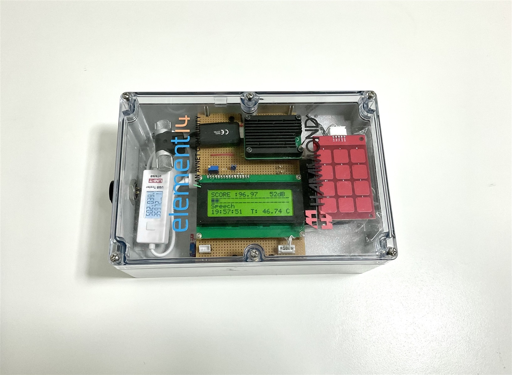
The screen is now divided into four lines of information:
- The first line displays the score, representing the probability score of the class identified in the sound classification process of the last 0.96 seconds processed. Additionally, it shows a relative value of decibels, indicating the maximum level of sound pressure referenced to a value obtained in silence. It's worth noting that this calibration is heuristic rather than scientific, as I lack the tools for precise calibration.
- The second line features a horizontal bar graph illustrating the sound pressure level in decibels, calculated using the root mean square (rms) of the last 1024 measurements. Sampling is conducted at 16 kHz, sampled values are 16 bits length integers.
- The third line displays the description of the class identified by the sound classifier, determined by the convolutional neural network. It indicates the class with the highest probability score within the last 0.96 seconds.
- The fourth line displays real-time updates obtained via NTP over the Wi-Fi connection, along with the CPU temperature of the Raspberry Pi4 compute module.
Me and Artificial Intelligence
In my academic years during the 80s and 90s, I delved into various facets of artificial intelligence (AI). One intriguing venture involved exploring fuzzy logic, a type of reasoning that handles approximate decisions rather than strict yes or no choices. Specifically, I applied fuzzy logic to enhance control systems for guiding vehicles in an automobile factory, where precise decisions weren't always feasible.
Another captivating project, sponsored by IBM, centered on crafting an expert system. These systems mimic human experts' decision-making skills within a specific field. My focus was on aiding lawyers with civil works claims by employing natural language processing to sift through legal documents and highlight potential breaches of contract. I utilized languages like Lisp, Prolog, and Crystal to build this rule-based system.
My journey into neural networks began with a research project involving predictions in a coal-fired power plant. Neural networks, adept at modeling complex behaviors, helped forecast power output based on factors like coal grinding levels and historical data.
Transitioning to my professional career, I ventured into developing an automated inventory replenishment system. Here, Bayesian inference played a pivotal role. This statistical method updates probabilities as new evidence emerges, aiding in predicting future sales based on past data and adjusting forecasts as sales evolve.
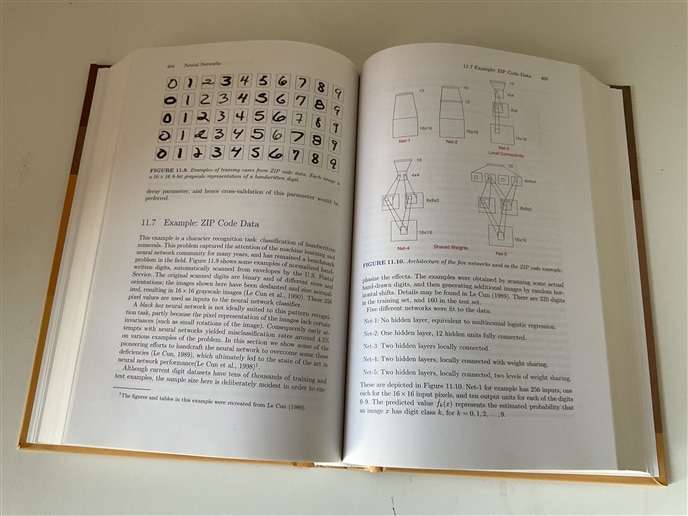
Throughout my career, statistical learning has remained a passion. I've recently revisited one of my favorite books on the subject: The Elements of Statistical Learning: Data Mining, Inference, and Prediction
Sound Feature Extraction and Classification
Feature extraction from sound data poses challenges. To make sense of raw sound data, we must distill it into more manageable forms. This entails extracting key features like frequency components and temporal patterns. By doing so, we create a structured representation that machine learning models can effectively interpret.
One method involves converting sound files into spectrograms, which visually represent frequency variations over time. These spectrograms serve as input for a model comprising a Convolutional Neural Network (CNN) paired with a Linear Classifier.
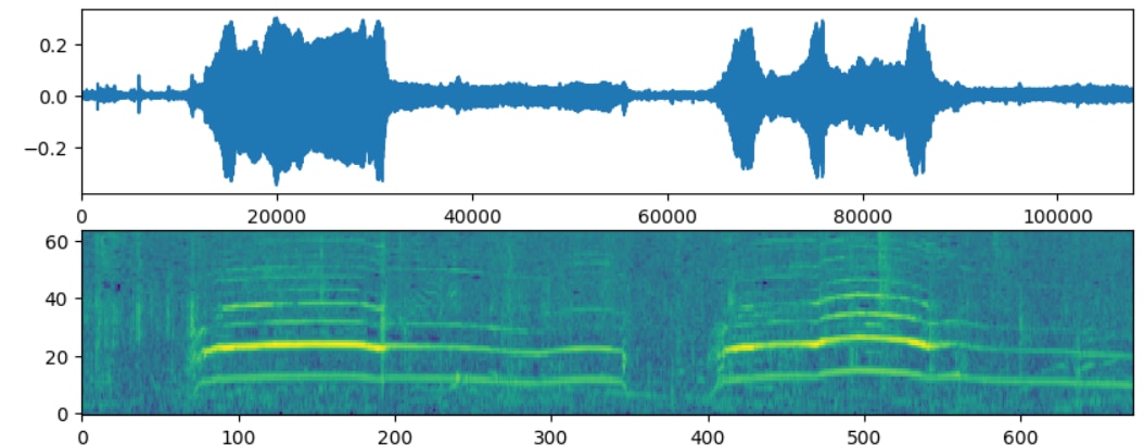
While CNNs are typically used for processing image data, they're also adept at handling sound spectrograms. These networks excel at recognizing patterns within grid-like data structures, making them suitable for sound analysis.
Ultimately, this model is employed to classify sound data into distinct categories based on its features.
Working with TensorFlow and Keras
For building the classification model, I've chosen to use TensorFlow with Keras. TensorFlow is an open-source machine learning framework developed by Google. TensorFlow can be used for various tasks such as classification, regression, clustering, and more. It allow us to define and train deep neural networks. Keras is the high-level API of the TensorFlow platform.


The TensorFlow development cycle begins with data preparation, followed by model design, where the neural network architecture is defined along with activation functions and the loss function chosen. Next, the model is trained using training data and evaluated for performance using test data. Hyperparameters, like learning rate, batch size, number of layers, activation functions.. are adjusted and the model is optimized as needed. Then we can deploy the model in real-world scenarios.
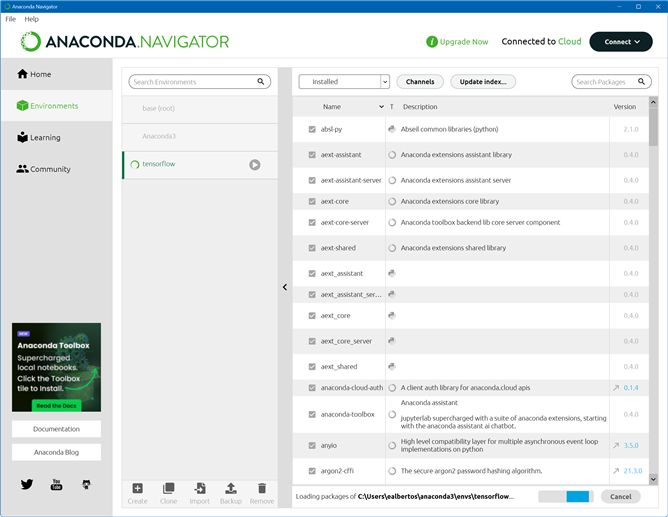
I've been working on Windows using Anaconda and JupyterLab notebooks.
Setting up the environment with Anaconda
Anaconda is a Python and R distribution that includes popular libraries and tools for data science and scientific computing.
To explore the dataset, analyze it, and build the model, we first need to set up the environment using Anaconda by creating a Python environment with the appropriate version for TensorFlow and the libraries we'll use for data exploration and analysis.

Creating the JupyterLab Notebook
Next, we need to create a notebook in JupyterLab, JupyterLab an interactive development environment for working with notebooks, code, and data.
The first thing we'll do is load the Python libraries we'll use throughout the notebook.
I used Librosa, a Python library for audio and music analysis. It provides tools for tasks such as loading audio files, extracting features from audio signals, and performing various audio processing tasks like pitch estimation, tempo detection, and spectrogram visualization.
Pandas is a Python library for data manipulation and analysis. It provides data structures and functions for handling structured data, such as tables and time series. NumPy provides support for large, multi-dimensional arrays and matrices, along with a collection of mathematical functions to operate on these arrays.
Seaborn and Matplotlib are Python data visualization libraries.
Keras, written in Python, is a high-level neural networks API that can be integrated with various machine learning frameworks, including TensorFlow.
Training a model from raw audio data
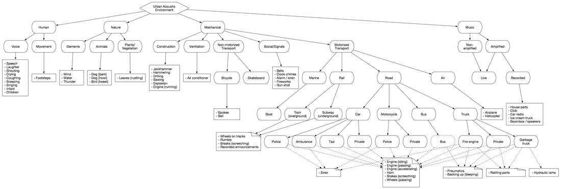
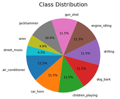
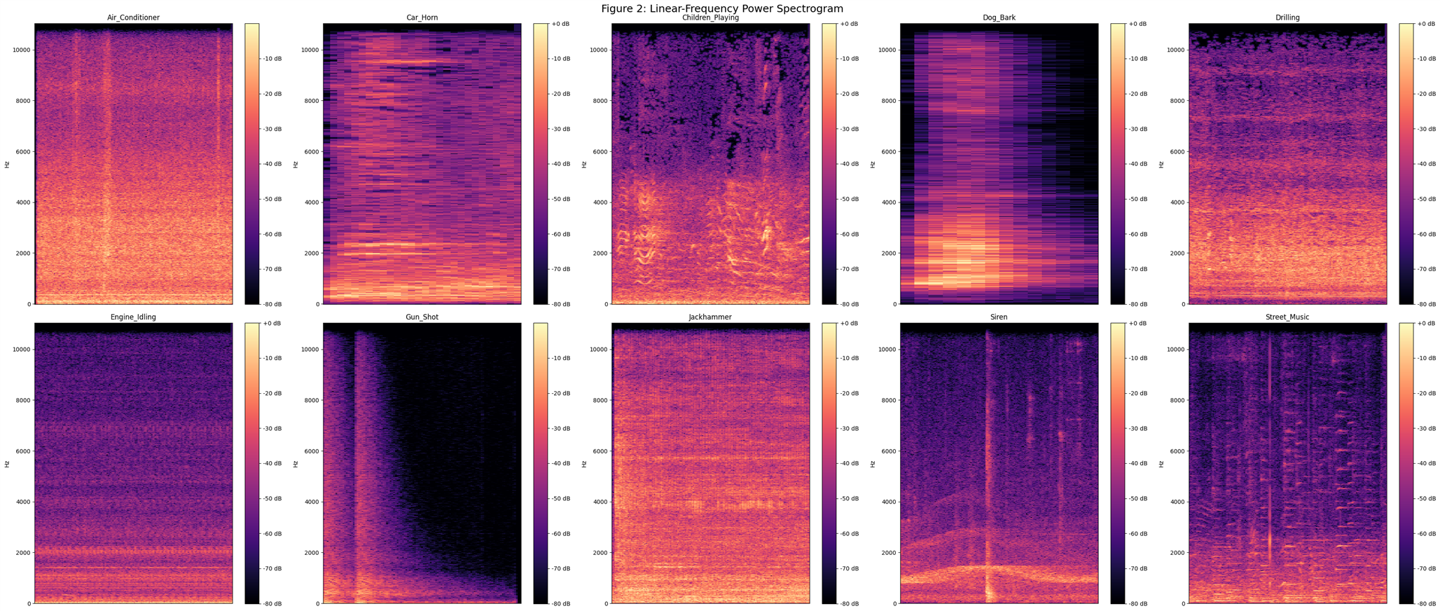
For this learning, I used a well-known dataset called UrbanSound8K . It contains 8732 labeled sound clips (<=4s) of urban sounds categorized into 10 classes: air_conditioner, car_horn, children_playing, dog_bark, drilling, engine_idling, gun_shot, jackhammer, siren, and street_music. These classes are based on the urban sound taxonomy. All clips are sourced from field recordings uploaded to freesound.org. Additionally, a CSV file with metadata for each clip is provided.
Exploring the UrbanSound8K dataset
After downloading the dataset, we see that it consists of two parts:
- Audio files in the ‘audio’ folder: It has 10 sub-folders named ‘fold1’ through ‘fold10’. Each sub-folder contains a number of ‘.wav’ audio samples eg. ‘fold1/103074–7–1–0.wav’,
- Metadata in the ‘metadata’ folder: It has a file ‘UrbanSound8K.csv’ that contains information about each audio sample in the dataset such as its filename, its class label, the ‘fold’ sub-folder location, and so on. The class label is a numeric Class ID from 0–9 for each of the 10 classes. eg. the number 0 means air conditioner, 1 is a car horn, and so on.
The meta-data contains 8 columns:
- slice_file_name: name of the audio file
- fsID: FreesoundID of the recording where the excerpt is taken from
- start: start time of the slice
- end: end time of the slice
- salience: salience rating of the sound.
- 1 = foreground,
- 2 = background
- fold: The fold number (1–10) to which this file has been allocated
- classID:
- 0 = air_conditioner
- 1 = car_horn
- 2 = children_playing
- 3 = dog_bark
- 4 = drilling
- 5 = engine_idling
- 6 = gun_shot
- 7 = jackhammer
- 8 = siren
- 9 = street_music
- class: class name
Exploring the metadata using python:
| slice_file_name | fsID | start | end | salience | fold | classID | class | |
|---|---|---|---|---|---|---|---|---|
| 0 | 100032-3-0-0.wav | 100032 | 0.000000 | 0.317551 | 1 | 5 | 3 | dog_bark |
| 1 | 100263-2-0-117.wav | 100263 | 58.500000 | 62.500000 | 1 | 5 | 2 | children_playing |
| 2 | 100263-2-0-121.wav | 100263 | 60.500000 | 64.500000 | 1 | 5 | 2 | children_playing |
| 3 | 100263-2-0-126.wav | 100263 | 63.000000 | 67.000000 | 1 | 5 | 2 | children_playing |
| 4 | 100263-2-0-137.wav | 100263 | 68.500000 | 72.500000 | 1 | 5 | 2 | children_playing |
| 5 | 100263-2-0-143.wav | 100263 | 71.500000 | 75.500000 | 1 | 5 | 2 | children_playing |
| 6 | 100263-2-0-161.wav | 100263 | 80.500000 | 84.500000 | 1 | 5 | 2 | children_playing |
| 7 | 100263-2-0-3.wav | 100263 | 1.500000 | 5.500000 | 1 | 5 | 2 | children_playing |
| 8 | 100263-2-0-36.wav | 100263 | 18.000000 | 22.000000 | 1 | 5 | 2 | children_playing |
| 9 | 100648-1-0-0.wav | 100648 | 4.823402 | 5.471927 | 2 | 10 | 1 | car_horn |
| slice_file_name | fsID | start | end | salience | fold | classID | class | |
|---|---|---|---|---|---|---|---|---|
| 8727 | 99812-1-2-0.wav | 99812 | 159.522205 | 163.522205 | 2 | 7 | 1 | car_horn |
| 8728 | 99812-1-3-0.wav | 99812 | 181.142431 | 183.284976 | 2 | 7 | 1 | car_horn |
| 8729 | 99812-1-4-0.wav | 99812 | 242.691902 | 246.197885 | 2 | 7 | 1 | car_horn |
| 8730 | 99812-1-5-0.wav | 99812 | 253.209850 | 255.741948 | 2 | 7 | 1 | car_horn |
| 8731 | 99812-1-6-0.wav | 99812 | 332.289233 | 334.821332 | 2 | 7 | 1 | car_horn |
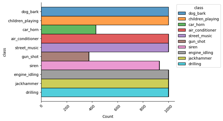
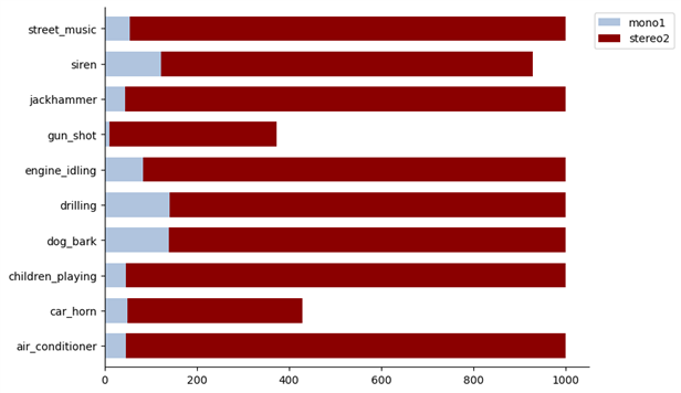
Audio Channels as can be observed, about 92% of the audio files are stereo, while the other 8% are mono.
The sampling rate of each of the samples is not homogeneous either.
| Sampling rate | Count |
| 44100 | 5370 |
| 48000 | 2502 |
| 96000 | 610 |
| 24000 | 82 |
| 16000 | 45 |
| 22050 | 44 |
| 192000 | 17 |
| 8000 | 12 |
| 11024 | 7 |
| 32000 | 4 |
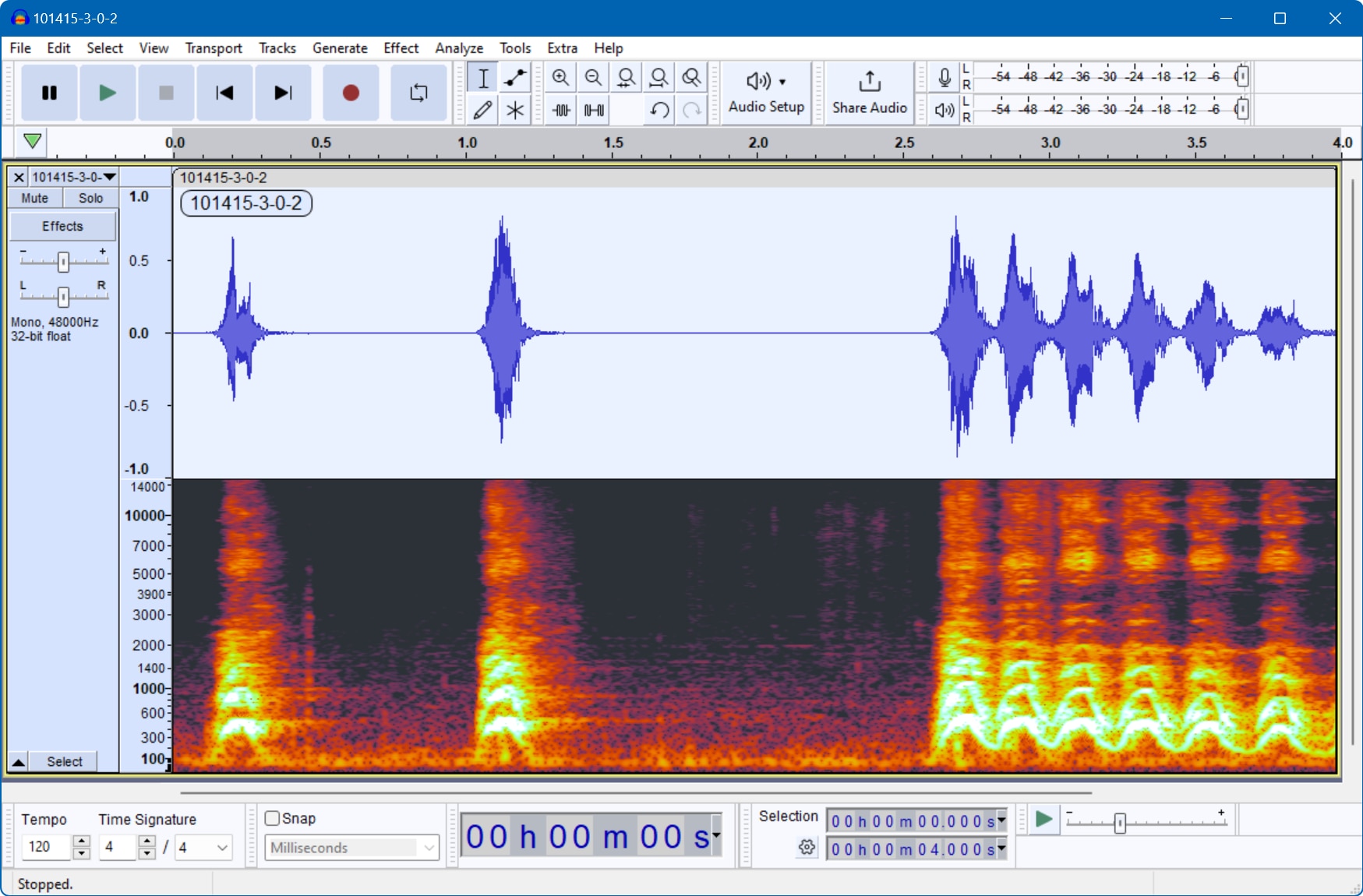
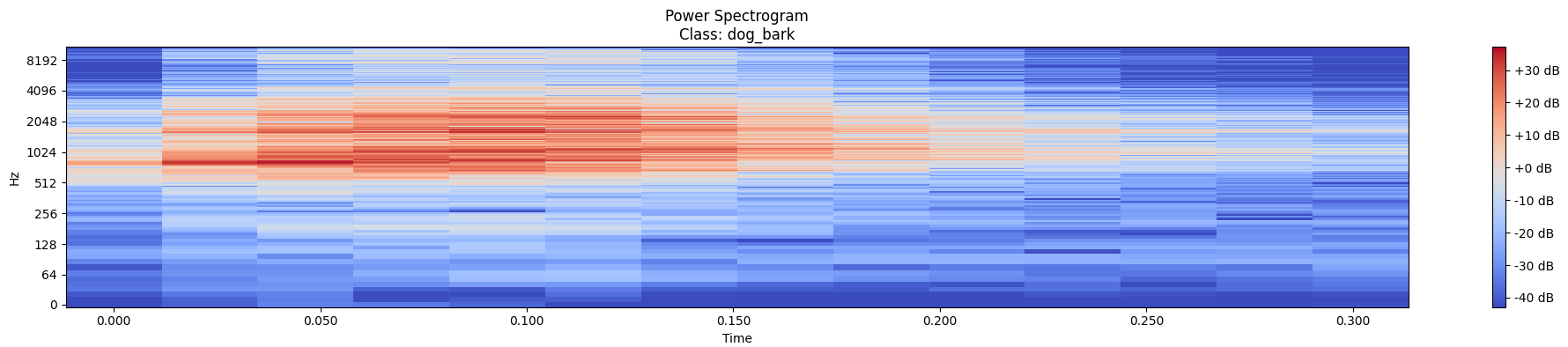
One example from the dataset, a dog bark:Analyzing the audio with Audacity. Audacity is a free software for recording and editing audio.
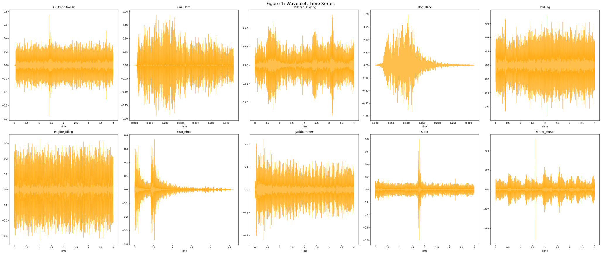
Short-time Fourier Transform (STFT)
To get that more granular view and see the frequency variations over time, we use the STFT algorithm (Short-Time Fourier Transform). The STFT is another variant of the Fourier Transform that breaks up the audio signal into smaller sections by using a sliding time window. It takes the FFT(Fast Fourier Transform) on each section and then combines them. It is thus able to capture the variations of the frequency with time.
Other Audio Representations
The power spectrogram is a visual representation of the frequency content of a signal over time. It displays how the energy of the signal is distributed across different frequency bands as it evolves over time. The spectrogram is obtained by applying the Fourier Transform to short overlapping segments of the signal, resulting in a time-frequency representation.
In a spectrogram, the x-axis represents time, the y-axis represents frequency, and the color intensity represents the magnitude of the signal's energy at each time-frequency bin.
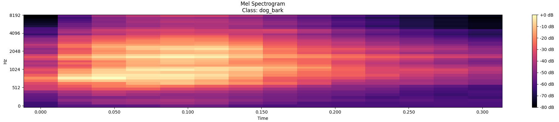
The Mel-spectrogram is a variation of the spectrogram where the frequency axis is transformed to the mel scale, which is a perceptual scale of pitches based on human hearing. The mel scale is nonlinear and better reflects how humans perceive the distance between different frequencies. Mel-spectrograms are commonly used in audio processing tasks, especially in speech and music analysis.
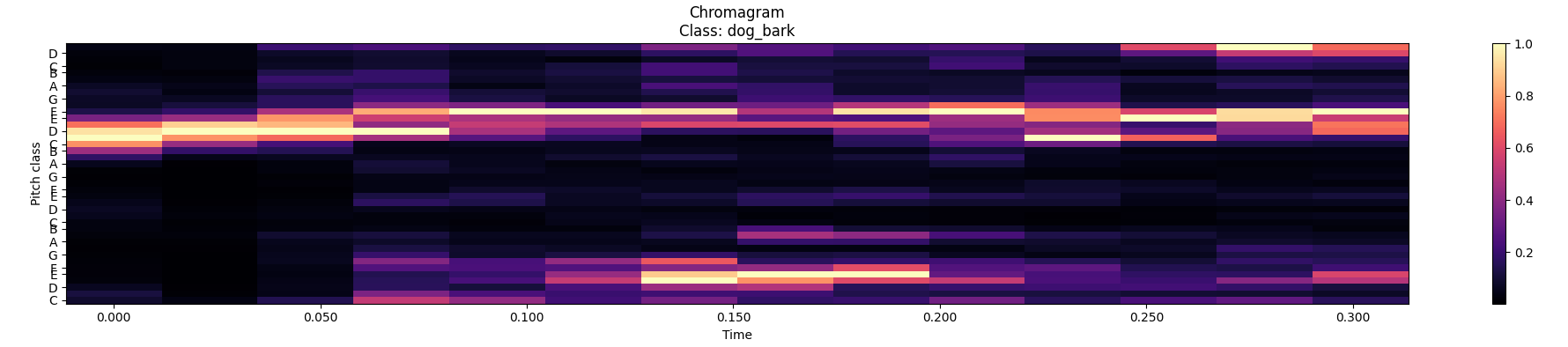
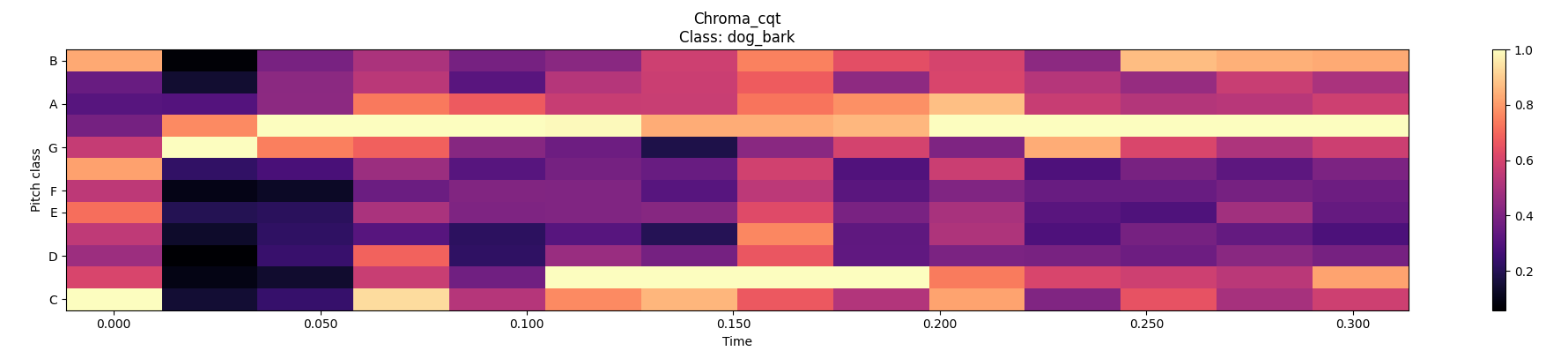
The chromagram, also known as a pitch class profile, is a representation of the pitch content of an audio signal over time. It divides the audio spectrum into 12 semitone-wide frequency bands, corresponding to the 12 pitch classes (C, C#, D, D#, E, F, F#, G, G#, A, A#, B). The chromagram is obtained by computing the energy or magnitude of the signal within each frequency band and then mapping it to the corresponding pitch class. Chromagrams are commonly used in music information retrieval tasks, such as genre classification, chord recognition, and melody extraction.
The Chroma CQT is a variant of the chromagram that uses the Constant-Q Transform (CQT) instead of the Fourier Transform. The CQT provides a logarithmically spaced frequency representation, which better matches the human auditory system's frequency resolution. Chroma CQT is particularly useful for analyzing audio signals with non-uniform frequency distributions, such as music recordings with varying harmonic content.
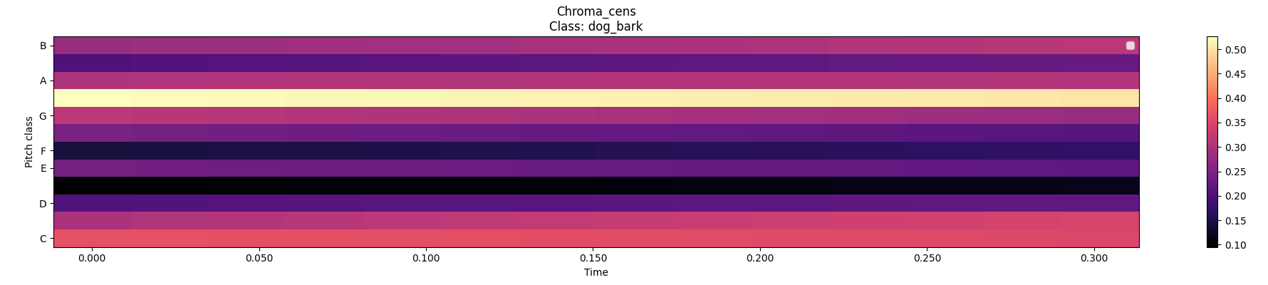
The Chroma CENS (Chroma Energy Normalized) is an extension of the chromagram that incorporates temporal smoothing and normalization to improve robustness to variations in audio dynamics and timbre. It applies smoothing techniques, such as median filtering or Gaussian filtering, to reduce the influence of transient events and noise. Additionally, chroma CENS normalizes the energy of each chroma vector across time, ensuring that variations in loudness or amplitude do not affect the chroma representation significantly.
Extracting features using mfcc
The librosa.feature.mfcc function in the Librosa library computes the Mel-frequency cepstral coefficients (MFCCs) of an audio signal.
mfccs = librosa.feature.mfcc(y=audio, sr=sample_rate, n_mfcc=40)
The output of librosa.feature.mfcc is a two-dimensional array of MFCC coefficients, where each row represents a different time frame and each column represents a different MFCC coefficient. By default, the function returns 20 MFCC coefficients (excluding the 0th coefficient, which represents the overall signal energy). However, the number of coefficients can be adjusted using the n_mfcc parameter.
The coefficients generated by the Mel-frequency cepstral coefficients (MFCCs) represent the characteristics of the power spectrum of an audio signal after processing through a series of transformations. The 0th coefficient typically represents the overall energy or power of the audio signal. It is computed as the logarithm of the total energy of the signal.
The remaining coefficients (C1 to Cn) capture spectral information about the audio signal, organized in the mel-frequency domain. Each coefficient represents the magnitude of the signal's power spectrum after filtering through a series of mel-frequency bands and applying a discrete cosine transform (DCT). These coefficients capture important features related to the frequency content of the signal, such as the distribution of energy across different frequency bands. The first few coefficients contain the most discriminative information, while higher-order coefficients capture more subtle spectral details.
Constructing the neural network
We constructed a convolutional neural network (CNN) using the Keras Sequential API with ReLU (Rectified Linear Unit) activation function for hidden layers and softmax activation function for the output layer.
model_relu = Sequential()
model_relu.add(Conv2D(filters=16, kernel_size=2, input_shape=(num_rows, num_columns, num_channels), activation='relu'))
model_relu.add(MaxPooling2D(pool_size=(2,2)))
model_relu.add(Dropout(0.2))

model_relu.add(Conv2D(filters=32, kernel_size=2, activation='relu'))
model_relu.add(MaxPooling2D(pool_size=(2,2)))
model_relu.add(Dropout(0.2))

model_relu.add(Conv2D(filters=64, kernel_size=2, activation='relu'))
model_relu.add(MaxPooling2D(pool_size=(2,2)))
model_relu.add(Dropout(0.2))

model_relu.add(Conv2D(filters=128, kernel_size=2, activation='relu'))
model_relu.add(MaxPooling2D(pool_size=(2,2)))
model_relu.add(Dropout(0.2))

model_relu.add(GlobalAveragePooling2D())
model_relu.add(Flatten())
model_relu.add(Dense(num_labels, activation='softmax'))

model_relu.compile(optimizer='adam', loss='categorical_crossentropy',
                   metrics=['accuracy'])
It uses convolutional layers for feature extraction, pooling layers for spatial downsampling, dropout layers for regularization, and fully connected layers for classification. It's a common CNN architecture used for image classification tasks in this case used for the sound spectrograms.
- Input Layer:
- Input shape: (num_rows, num_columns, num_channels) - Specifies the shape of the input data, where num_rows and num_columns represent the height and width of the input
- images, and num_channels represents the number of color channels (e.g., 3 for RGB images).
- Conv2D layer with 16 filters and a kernel size of 2x2, using ReLU activation function.
- MaxPooling2D layer with a pool size of 2x2, which reduces the spatial dimensions of the feature maps by a factor of 2.
- The four sets of Conv2D layers followed by MaxPooling2D layers and Dropout layers:
- Conv2D layer with 32 filters and a kernel size of 2x2, using ReLU activation function.
- MaxPooling2D layer with a pool size of 2x2.
- Dropout layer with a dropout rate of 0.2.
- GlobalAveragePooling2D layer averages the values in each feature map, resulting in a single value per feature map
- Flatten layer converts the 2D feature maps into a 1D vector, preparing the data for the fully connected layers.
- Output Layer: Dense layer with num_labels units (number of classes) and softmax activation function. Softmax function is commonly used in classification tasks to output probability distribution over multiple classes.
- Compilation:
- Adam optimizer is used with categorical cross-entropy loss, which is suitable for multi-class classification tasks.
- Metrics are specified as accuracy to monitor model performance during training.
Summary:
Model: "sequential"
_________________________________________________________________
 Layer (type)                Output Shape              Param #
=================================================================
 conv2d (Conv2D)             (None, 39, 173, 16)       80
 max_pooling2d (MaxPooling2  (None, 19, 86, 16)        0
 D)
 dropout (Dropout)           (None, 19, 86, 16)        0
 conv2d_1 (Conv2D)           (None, 18, 85, 32)        2080
 max_pooling2d_1 (MaxPoolin  (None, 9, 42, 32)         0
 g2D)
 dropout_1 (Dropout)         (None, 9, 42, 32)         0
 conv2d_2 (Conv2D)           (None, 8, 41, 64)         8256
 max_pooling2d_2 (MaxPoolin  (None, 4, 20, 64)         0
 g2D)
 dropout_2 (Dropout)         (None, 4, 20, 64)         0
 conv2d_3 (Conv2D)           (None, 3, 19, 128)        32896
 max_pooling2d_3 (MaxPoolin  (None, 1, 9, 128)         0
 g2D)
 dropout_3 (Dropout)         (None, 1, 9, 128)         0
 global_average_pooling2d (  (None, 128)               0
 GlobalAveragePooling2D)
 flatten (Flatten)           (None, 128)               0
 dense (Dense)               (None, 10)                1290
=================================================================
Total params: 44602 (174.23 KB)
Trainable params: 44602 (174.23 KB)
Non-trainable params: 0 (0.00 Byte)
_________________________________________________________________
Preparing the audio data
Audio data must be prepared, resampled and converted to mono and to the same sample rate and then normalized.
Training the model
First, we split the dependent and independent features. After that, we have 10 classes, so we use label encoding(Integer label encoding) from number 1 to 10 and convert it into categories. After that, Now, we split the dataset into training, validation and test datasets. In general, the ratio for splitting is 80% for training, 10% for validation and 10% for test sets.
num_epochs = 400
num_batch_size = 256

checkpointer = ModelCheckpoint(filepath='saved_models/weights.best.basic_cnn_v2.hdf5',
                               verbose=1, save_best_only=True)
start = datetime.now()

history_relu = model_relu.fit(X_train, y_train, batch_size=num_batch_size, epochs=num_epochs, validation_data = (X_test, y_test), callbacks=[checkpointer], verbose=1)

duration = datetime.now() - start
print("Training completed in time: ", duration)
Then run the training
Epoch 1/400
28/28 [==============================] - ETA: 0s - loss: 3.9066 - accuracy: 0.1784
Epoch 1: val_loss improved from inf to 2.11179, saving model to saved_models\weights.best.basic_cnn_v2.hdf5
28/28 [==============================] - 8s 252ms/step - loss: 3.9066 - accuracy: 0.1784 - val_loss: 2.1118 - val_accuracy: 0.1808
Epoch 2/400
28/28 [==============================] - ETA: 0s - loss: 1.8893 - accuracy: 0.3204
Epoch 2: val_loss improved from 2.11179 to 1.87491, saving model to saved_models\weights.best.basic_cnn_v2.hdf5
28/28 [==============================] - 7s 251ms/step - loss: 1.8893 - accuracy: 0.3204 - val_loss: 1.8749 - val_accuracy: 0.3776
Epoch 3/400
28/28 [==============================] - ETA: 0s - loss: 1.6222 - accuracy: 0.4210
Epoch 3: val_loss improved from 1.87491 to 1.68137, saving model to saved_models\weights.best.basic_cnn_v2.hdf5
28/28 [==============================] - 7s 245ms/step - loss: 1.6222 - accuracy: 0.4210 - val_loss: 1.6814 - val_accuracy: 0.4600
Epoch 4/400
28/28 [==============================] - ETA: 0s - loss: 1.4780 - accuracy: 0.4825
Epoch 4: val_loss improved from 1.68137 to 1.57626, saving model to saved_models\weights.best.basic_cnn_v2.hdf5
28/28 [==============================] - 7s 251ms/step - loss: 1.4780 - accuracy: 0.4825 - val_loss: 1.5763 - val_accuracy: 0.4840
Epoch 5/400
28/28 [==============================] - ETA: 0s - loss: 1.3704 - accuracy: 0.5248
Epoch 5: val_loss improved from 1.57626 to 1.47619, saving model to saved_models\weights.best.basic_cnn_v2.hdf5
28/28 [==============================] - 7s 248ms/step - loss: 1.3704 - accuracy: 0.5248 - val_loss: 1.4762 - val_accuracy: 0.5286
...
...
28/28 [==============================] - ETA: 0s - loss: 0.0531 - accuracy: 0.9828
Epoch 387: val_loss did not improve from 0.19665
28/28 [==============================] - 7s 250ms/step - loss: 0.0531 - accuracy: 0.9828 - val_loss: 0.2363 - val_accuracy: 0.9336
Epoch 388/400
28/28 [==============================] - ETA: 0s - loss: 0.0379 - accuracy: 0.9863
Epoch 388: val_loss improved from 0.19665 to 0.18787, saving model to saved_models\weights.best.basic_cnn_v2.hdf5
28/28 [==============================] - 7s 264ms/step - loss: 0.0379 - accuracy: 0.9863 - val_loss: 0.1879 - val_accuracy: 0.9451
Epoch 389/400
28/28 [==============================] - ETA: 0s - loss: 0.0335 - accuracy: 0.9877
Epoch 389: val_loss did not improve from 0.18787
28/28 [==============================] - 7s 258ms/step - loss: 0.0335 - accuracy: 0.9877 - val_loss: 0.2795 - val_accuracy: 0.9359
Epoch 390/400
28/28 [==============================] - ETA: 0s - loss: 0.0347 - accuracy: 0.9878
Epoch 390: val_loss did not improve from 0.18787
28/28 [==============================] - 7s 259ms/step - loss: 0.0347 - accuracy: 0.9878 - val_loss: 0.2092 - val_accuracy: 0.9428
Epoch 391/400
28/28 [==============================] - ETA: 0s - loss: 0.0414 - accuracy: 0.9855
Epoch 391: val_loss did not improve from 0.18787
28/28 [==============================] - 7s 256ms/step - loss: 0.0414 - accuracy: 0.9855 - val_loss: 0.2176 - val_accuracy: 0.9359
Epoch 392/400
28/28 [==============================] - ETA: 0s - loss: 0.0463 - accuracy: 0.9837
Epoch 392: val_loss did not improve from 0.18787
28/28 [==============================] - 7s 253ms/step - loss: 0.0463 - accuracy: 0.9837 - val_loss: 0.2444 - val_accuracy: 0.9314
Epoch 393/400
28/28 [==============================] - ETA: 0s - loss: 0.0442 - accuracy: 0.9841
Epoch 393: val_loss did not improve from 0.18787
28/28 [==============================] - 7s 252ms/step - loss: 0.0442 - accuracy: 0.9841 - val_loss: 0.2598 - val_accuracy: 0.9348
Epoch 394/400
28/28 [==============================] - ETA: 0s - loss: 0.0470 - accuracy: 0.9845
Epoch 394: val_loss did not improve from 0.18787
28/28 [==============================] - 7s 250ms/step - loss: 0.0470 - accuracy: 0.9845 - val_loss: 0.2440 - val_accuracy: 0.9428
Epoch 395/400
28/28 [==============================] - ETA: 0s - loss: 0.0440 - accuracy: 0.9855
Epoch 395: val_loss did not improve from 0.18787
28/28 [==============================] - 7s 254ms/step - loss: 0.0440 - accuracy: 0.9855 - val_loss: 0.2175 - val_accuracy: 0.9359
Epoch 396/400
28/28 [==============================] - ETA: 0s - loss: 0.0429 - accuracy: 0.9848
Epoch 396: val_loss did not improve from 0.18787
28/28 [==============================] - 7s 248ms/step - loss: 0.0429 - accuracy: 0.9848 - val_loss: 0.2459 - val_accuracy: 0.9359
Epoch 397/400
28/28 [==============================] - ETA: 0s - loss: 0.0361 - accuracy: 0.9870
Epoch 397: val_loss did not improve from 0.18787
28/28 [==============================] - 7s 250ms/step - loss: 0.0361 - accuracy: 0.9870 - val_loss: 0.2963 - val_accuracy: 0.9336
Epoch 398/400
28/28 [==============================] - ETA: 0s - loss: 0.0410 - accuracy: 0.9864
Epoch 398: val_loss did not improve from 0.18787
28/28 [==============================] - 7s 242ms/step - loss: 0.0410 - accuracy: 0.9864 - val_loss: 0.2785 - val_accuracy: 0.9394
Epoch 399/400
28/28 [==============================] - ETA: 0s - loss: 0.0424 - accuracy: 0.9835
Epoch 399: val_loss did not improve from 0.18787
28/28 [==============================] - 7s 253ms/step - loss: 0.0424 - accuracy: 0.9835 - val_loss: 0.2597 - val_accuracy: 0.9336
Epoch 400/400
28/28 [==============================] - ETA: 0s - loss: 0.0488 - accuracy: 0.9821
Epoch 400: val_loss did not improve from 0.18787
28/28 [==============================] - 7s 252ms/step - loss: 0.0488 - accuracy: 0.9821 - val_loss: 0.2262 - val_accuracy: 0.9416
Training completed in time:  0:48:00.924988
It took me 48 minutes on my computer using the CPU since the latest versions of TensorFlow on Windows do not support GPU.
Evaluating the model with the loss function
The primary goal of the loss function is to guide the optimization process during training by providing a measure of how well the model is performing on the training data.
We have used categorical cross-entropy, this loss function is commonly used in multi-class classification tasks where the output consists of probabilities assigned to multiple classes.
It measures the dissimilarity between the true probability distribution of the labels and the predicted probability distribution produced by the model.
Categorical cross-entropy encourages the model to assign higher probabilities to the correct class labels while penalizing deviations from the true distribution.
# Evaluating the model on the training and testing set:
score = model_relu.evaluate(X_train, y_train, verbose=0)
print("Training Accuracy: ", score[1])

score = model_relu.evaluate(X_test, y_test, verbose=0)
print("Testing Accuracy: ", score[1])

Training Accuracy:  0.9985683560371399
Testing Accuracy:  0.9416475892066956

# Plotting Loss of CNN 2D - ReLu Model:
metrics = history_relu.history

plt.plot(history_relu.epoch, metrics['loss'], metrics['val_loss'])
plt.legend(['train_loss', 'test_loss'])

plt.xlabel('Epoch')
plt.ylabel('Loss')

plt.legend([])
plt.grid(True)
plt.savefig("loss")
plt.show()
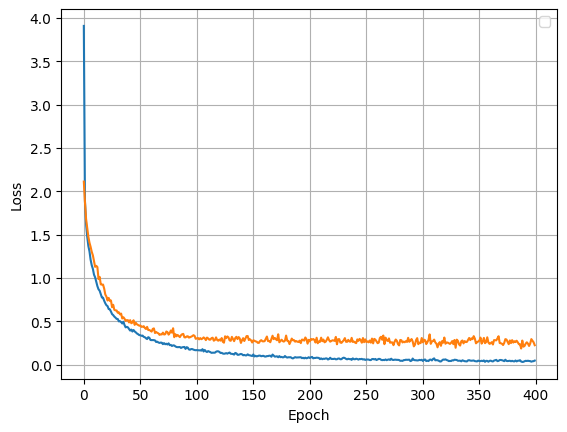
The loss function decreases with each epoch and there is no overfitting.
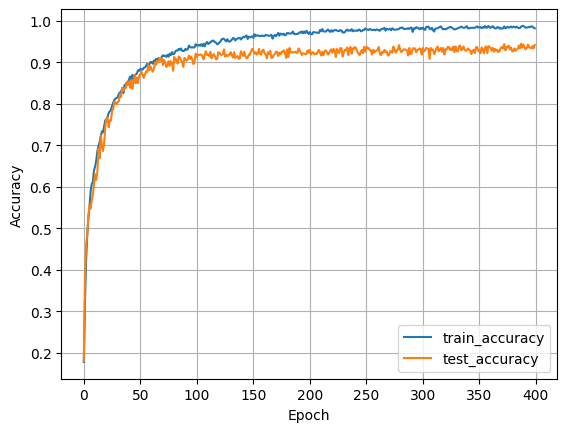
Model Accuracy
The accuracy measures the proportion of correctly classified samples among the total number of samples in the dataset.
- Accuracy is calculated as the ratio of the number of correctly predicted samples to the total number of samples in the dataset.
- Mathematically, accuracy is expressed as:
Accuracy = Number of Correct Predictions / Total Number of Predictions
# Plotting Accuracy of CNN 2D - ReLu Model:
plt.plot(metrics['accuracy'], label='train_accuracy')
plt.plot(metrics['val_accuracy'], label='test_accuracy')

plt.xlabel('Epoch')
plt.ylabel('Accuracy')

plt.legend()
plt.grid(True)
plt.savefig("accuracy")
plt.show()
Performance metrics of the model
test_result = model_relu.test_on_batch(X_test, y_test)
print(test_result)
[0.2262222021818161, 0.9416475892066956]
In this project we have 94% accuracy with 0.226 loss.
Testing the model
Finally I tested the model, that works really well.
def prediction_(path_file):
    data_sound = extract_features(path_file)
    X = np.array(data_sound)
    pred_result = model_relu.predict(X.reshape(1,40,174,1))
    pred_class = pred_result.argmax()
    pred_prob = pred_result.max()
    print(f"This belongs to class {pred_class} : {classes[int(pred_class)]}  with {pred_prob} probability")

prediction_(metadata.path_file[500])
ipd.Audio(metadata.path_file[500])
arr = np.array(metadata["slice_file_name"])
fold = np.array(metadata["fold"])
cla = np.array(metadata["classID"])
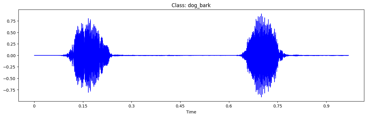
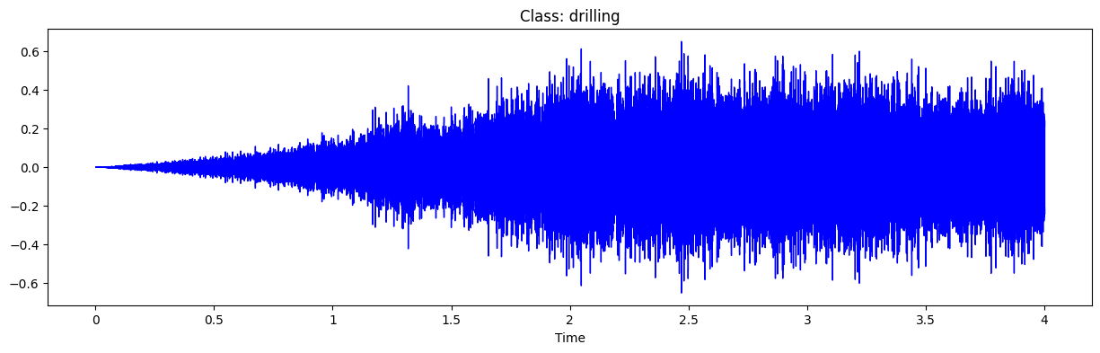
for i in range(192, 197, 2):
path = path_audio+'fold' + str(fold[i]) + '/' + arr[i]
prediction_(path)
y, sr = librosa.load(path)
plt.figure(figsize=(15,4))
plt.title('Class: '+classes[int(cla[i])])
librosa.display.waveshow(y, sr=sr, color='blue')
ipd.Audio(path)
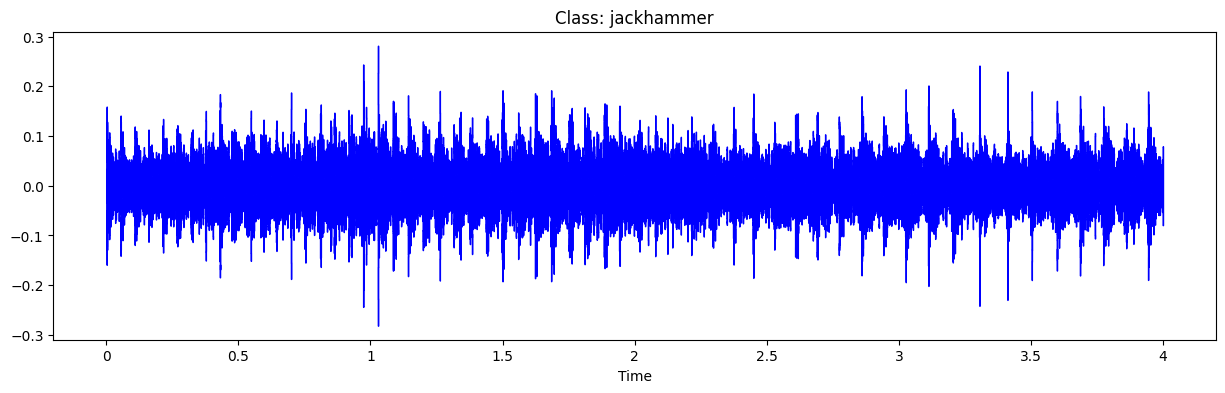
1/1 [==============================] - 0s 40ms/step
This belongs to class 7 : jackhammer  with 0.9991942048072815 probability


1/1 [==============================] - 0s 30ms/step
This belongs to class 3 : dog_bark with 1.0 probability


1/1 [==============================] - 0s 30ms/step
This belongs to class 4 : drilling with 0.9999679327011108 probability
Exploring Neural Networks with Keras and TensorFlow: Lessons Learned and Next Steps
I used tools like Keras and TensorFlow, which are really handy for building neural networks easily and efficiently. The model I made using the UrbanSound dataset turned out to work pretty well. However, I overlooked something important for my project - classifying silence. I realized this later on, but it's not too hard to fix; I just need to add a new category for silence.
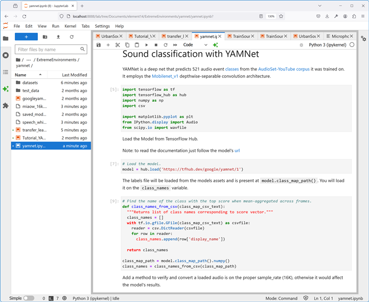
But, I've decided to try something different. I want to test out another model that's already been trained. It's called Yamnet, and it's made by Google. I'll explain more about it in the next part
Using a pretrained model. The Google YAMnet
After experimenting with a couple of models built from scratch using the UrbanSound8K dataset, I stumbled upon a pre-trained model developed by Google. Intrigued by its potential, I decided to give it a try. To my surprise, the results on my Windows machine were impressive.
Encouraged by this success, I proceeded to port the predictor to the Raspberry Pi. Using the PyAudio library for the PortAudio v19 audio I/O library, I captured sound with the microphone and integrated it with the libraries I had previously created for the LCD display driver and the capacitive keyboard.
YAMnet, short for Yet Another Multilabel Network, is a deep learning model developed by Google for sound event recognition. YAMNet is an audio event classifier that takes audio waveform as input and makes independent predictions for each of 521 audio events from the AudioSet ontology.
Started with this Yamnet Tutorial. https://colab.research.google.com/github/tensorflow/docs/blob/master/site/en/hub/tutorials/yamnet.ipynb
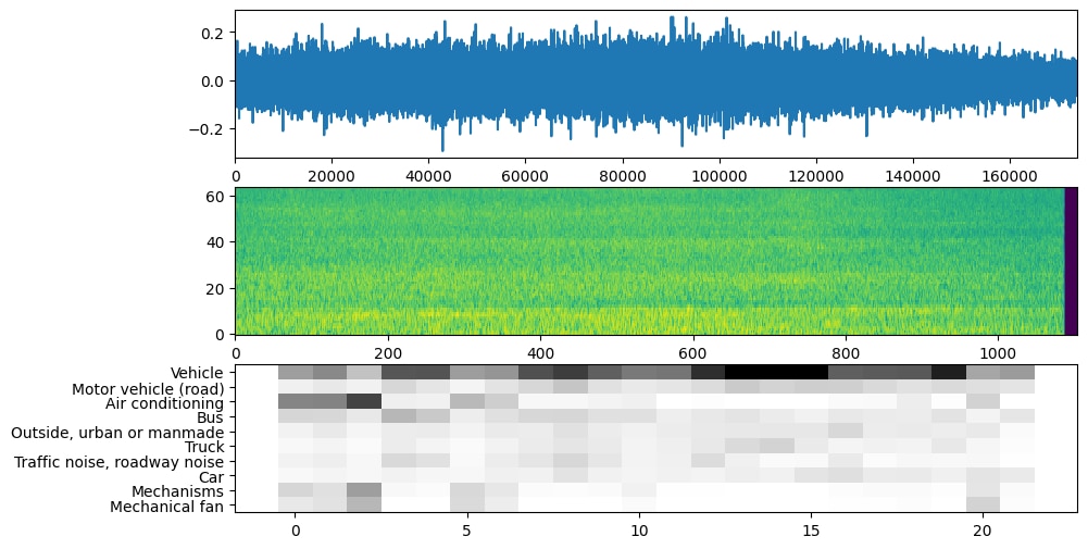
Let see some examples of the prediction outputs using this model.
First audio captured with the Raspberry Pi4 Compute Module and the Trust Microphone + USB Audio card
An example given by Google
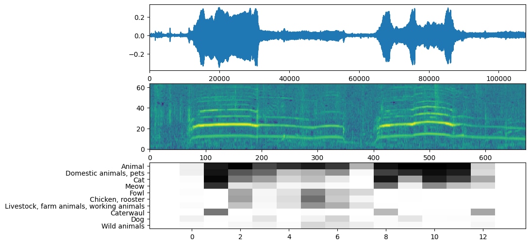
Another sound captured with the Raspberry Pi4 Compute Module and the Trust Microphone + USB Audio card
Python code
import tensorflow as tf
import tensorflow_hub as hub
import numpy as np
import csv


from scipy.io import wavfile

# Load the model.
# model = hub.load('https://tfhub.dev/google/yamnet/1')
model = hub.load('./yamnet_model')


# Find the name of the class with the top score when mean-aggregated across frames.
def class_names_from_csv(class_map_csv_text):
  """Returns list of class names corresponding to score vector."""
  class_names = []
  with tf.io.gfile.GFile(class_map_csv_text) as csvfile:
    reader = csv.DictReader(csvfile)
    for row in reader:
      class_names.append(row['display_name'])

  return class_names

class_map_path = model.class_map_path().numpy()
class_names = class_names_from_csv(class_map_path)

def ensure_sample_rate(original_sample_rate, waveform,
                       desired_sample_rate=16000):
  """Resample waveform if required."""
  if original_sample_rate != desired_sample_rate:
    desired_length = int(round(float(len(waveform)) /
                               original_sample_rate * desired_sample_rate))
    waveform = scipy.signal.resample(waveform, desired_length)
  return desired_sample_rate, waveform


wav_file_name = 'recycling_truck.wav'

sample_rate, wav_data = wavfile.read(wav_file_name, 'rb')
sample_rate, wav_data = ensure_sample_rate(sample_rate, wav_data)

# Show some basic information about the audio.
duration = len(wav_data)/sample_rate
print(f'Sample rate: {sample_rate} Hz')
print(f'Total duration: {duration:.2f}s')
print(f'Size of the input: {len(wav_data)}')

# Listening to the wav file.
Audio(wav_data, rate=sample_rate)

# The wav_data needs to be normalized to values in [-1.0, 1.0]
waveform = wav_data / tf.int16.max

# Run the model, check the output.
scores, embeddings, spectrogram = model(waveform)

scores_np = scores.numpy()
spectrogram_np = spectrogram.numpy()
infered_class = class_names[scores_np.mean(axis=0).argmax()]
print(f'The main sound is: {infered_class}')
Installing TensorFlow on the Raspberry Pi4 Compute Module
Preparing the Python environment to run the sound classifier on the Raspberry Pi is very simple.
https://www.tensorflow.org/install/pip?lang=python3
python -m venv --system-site-packages pyenv
sudo apt-get install libhdf5-serial-dev

python3 -m pip install tensorflow
python3 -m pip install tensorflow_hub
It is a large installation
Installing PyAudio
PyAudio provides Python bindings for PortAudio v19, the cross-platform audio I/O library. With PyAudio, you can easily use Python to play and record audio on a variety of platforms, such as GNU/Linux, Microsoft Windows, and Apple macOS.
First install PortAudio v19
sudo apt-get install portaudio19-dev
Then in your python environment pip install pyAudio
pip install PyAudio
Insall scipy
pip install scipy
Using Alsamixer to set microphone gain
alsamixer is a command-line audio mixer utility for the Advanced Linux Sound Architecture (ALSA) system, which is commonly used in Linux-based operating systems.
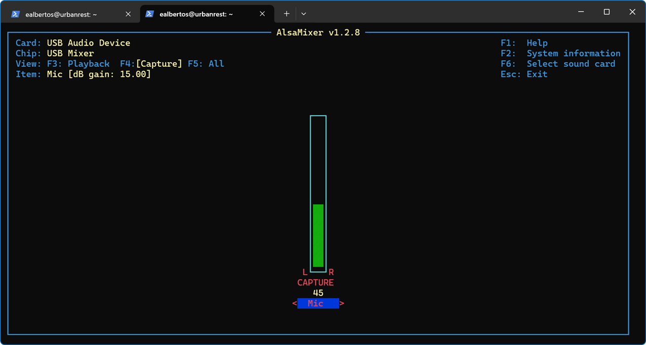
It provides a graphical interface within the terminal for adjusting various audio settings, such as volume levels, input/output selection, and channel balance.
We utilize it to adjust the microphone capture gain level, a critical aspect for our project. This adjustment determines what qualifies as silence and helps us prevent microphone saturation.
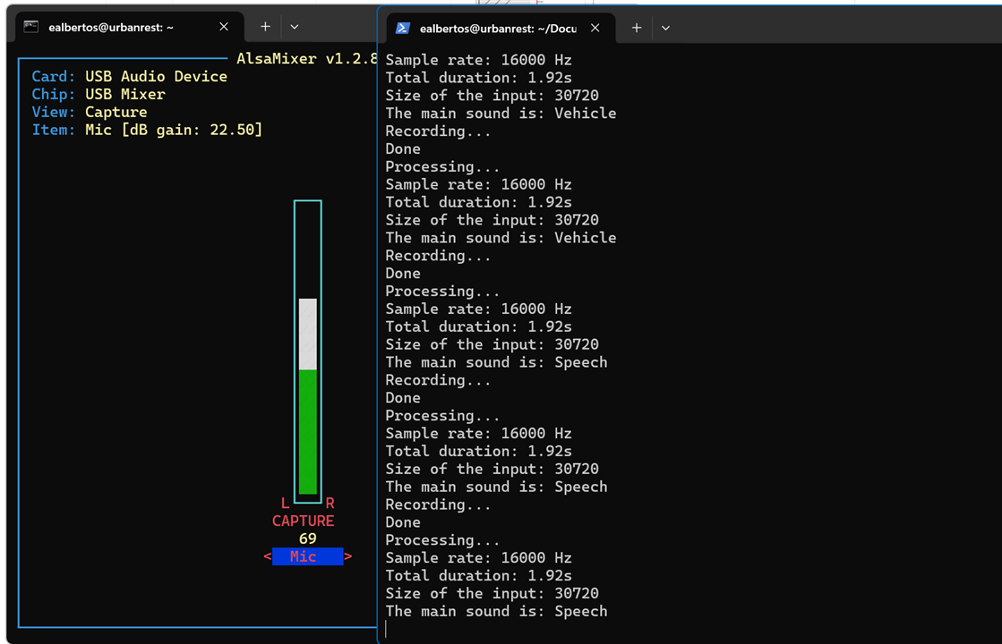
Field tests with the YAMnet model
Many of the tests conducted revolve around determining the feasibility of housing the microphone inside the box. Understandably, the acoustics inside the box differ, with more reverberation present. This often results in periods of silence, indicating that the microphone is situated within a confined space, essentially a box.
Moreover, it appears that the foam used to bed the battery improves the sound conditions. While increasing the microphone gain can partially compensate for the acoustic isolation provided by the box, it also amplifies signal noise.
Siren rising from https://freesound.org/
Street parade with music
Urban ambience. People talking
Pocket radio tuning
Night street sound
Summary and conclusions
After two weeks of experimentation, I'm thrilled with the excellent results. I had prior experience with sound recognition using TensorFlow Lite, but I couldn't achieve such impressive outcomes. It seems my hand injury is getting worse, soI still need to wait before finishing machining the box to attach the microphone externally.
Thanks for reading!
UrbanRest Guardian blog series
Want to know more about this project? Check out the full blog series here:
- Blog 1 - UrbanRest Guardian - Project Introduction
- Blog 2 - UrbanRest Guardian - First contact with the kit components.
- Blog 3 - UrbanRest Guardian - Prototype Construction Journey
- Blog 4 - UrbanRest Guardian - Classifying Urban Sounds
- Blog 5 - UrbanRest Guardian - Remote Monitoring
- Final Blog - UrbanRest Guardian - Smart Street Noise Monitor
-

genebren
-
Cancel
-
Vote Up
0
Vote Down
-
-
Sign in to reply
-
More
-
Cancel
-

javagoza
in reply to genebren
-
Cancel
-
Vote Up
0
Vote Down
-
-
Sign in to reply
-
More
-
Cancel
Comment-

javagoza
in reply to genebren
-
Cancel
-
Vote Up
0
Vote Down
-
-
Sign in to reply
-
More
-
Cancel
Children