My ADI ADALM2000 device, received under Element14's Roadtest program, came at a time when I had begun working on a project related to communications on relatively long (few kilometers long) twisted pairs. I have used cables in different projects in the past, but never this long. For many of the normal use cases we view the cables as conductors and don't worry too much about the rest. However, as the length starts getting longer, you can no longer ignore the cable characteristics. I saw this as a good opportunity to learn more about the behaviour of cables and transmission lines.

Since the ADALM2000 includes several instruments inside (the most relevant in this case being (2x)Function generators, (2x) oscilloscope channels and the necessary software to also function as Spectrum analyzer and Network Analyzer), this gave me the tools I needed to explore cable characteristics in the Time and Frequency domains. 

Twisted pairs as Transmission Lines

From my limited understanding so far, at DC and very low frequencies, thinking of cables as conductors with some resistance per unit length works just fine. Characteristics like cable's characteristic impedance don't matter too much if you're just using it to transmit some DC power or signals are very low frequencies. However, as our operating frequencies start to increase into the tens of kHz or MHz (or higher) frequencies, we can no longer keep that simplistic view of cables. This becomes even more important when we transmit our signals over longer distances.

One important detail to keep in mind about twisted pairs is that, when used in communications, they are used to carry differential signals, not single ended signals. In differential signalling the two wires in the pair are carrying equal but opposite signals at any instance in time. This is different than the case of "single ended" singalling, where one conductor is carrying the signal while the other conductor is grounded. Coaxial cables are a very common example of single-ended signalling whereby the center conductor carries the signals while the outer shielding conductor is grounded. Twisted pairs, like those in Ethernet cables, use differential signalling.

Test Setup

For these tests, I will be using 2 x15 meter long twisted-pair cables. Joining them back to back gives me 30m of twisted pair cabling. The cables already have DB9 connectors installed on both sides, connected to pins 1&2. I have soldered mating connectors to small lengths of similar twisted pair wires to make connections.

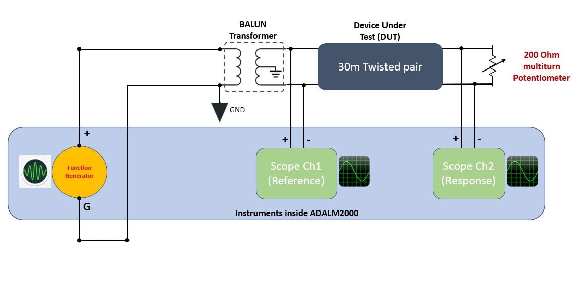
As mentioned, my tool of choice for these experiments is the ADI ADALM2000. I will be using the Function generator inside the ADALM2000 to "launch" signals into the cable and the Oscilloscope channels to measure responses. The Scopy software will do the magic to let me explore in time and frequency domains.

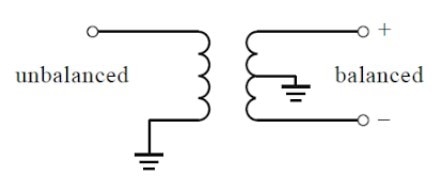
One thing to note is that the function generator inside the ADALM2000 is single ended (a.k.a "ground referenced" or "unbalanced"). Since our Device-Under-Test (Twisted pair cable) works with differential signals, we need to convert our single ended signals to differential signals (a.k.a "balanced" signals). The device to accomplish this is called a BALUN, which is basically a transformer. I encourage you to read the Wikipedia article for a better understanding. The name BALUN is derived from BAL (Balanced) UN (unbalanced).

I was able to find a balun that works in the 10kHz to 60MHz range, which is good enough for my use. Ideally the output impedance of the BALUN on the differential side (125 Ohms in my case) should match that of the connected DUT. I don't know my cable's characteristic impedance (probably 100Ohms), but since this is the only BALUN available to me anyway, so I'll just go with this.

With the stimulus signal converted to differential on one side of the cable/transmission line, and received on the other side in differential mode as well, we can use the Oscilloscope channels inside the ADALM2000, which are differential in nature, to capture the stimulus and response signals on both sides of the Device Under Test (DUT) - cable.

The final connection diagram is as following:

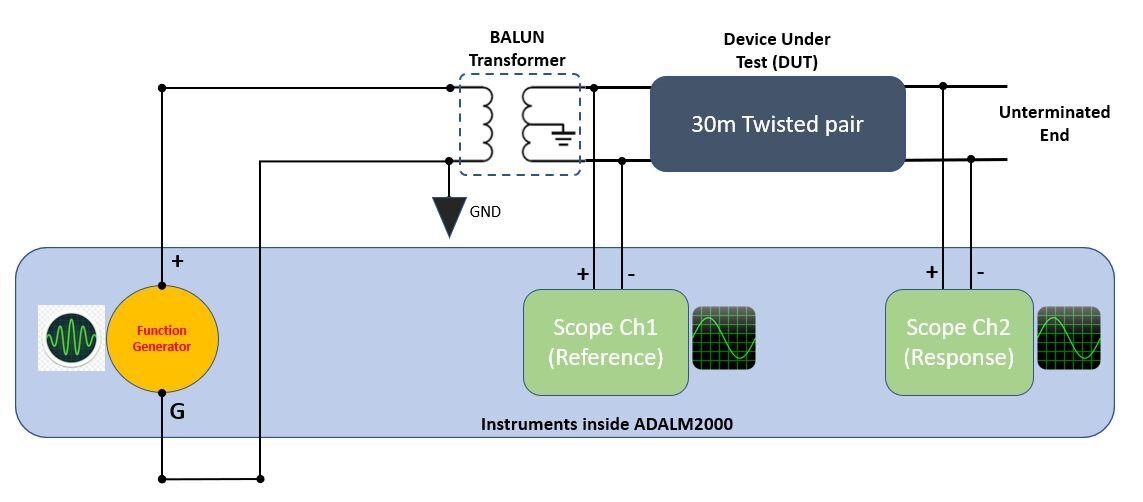
Note that the "reference" scope channel is connected AFTER the BALUN. This is to ignore any effects introduced by the BALUN, so that we only measure what goes into (and comes out of) the cable. Also notice that for this test we have the far end of the cable unterminated, i.e., without any load. This is intentionally done to cause reflections of signal from the far end, as we will see later.

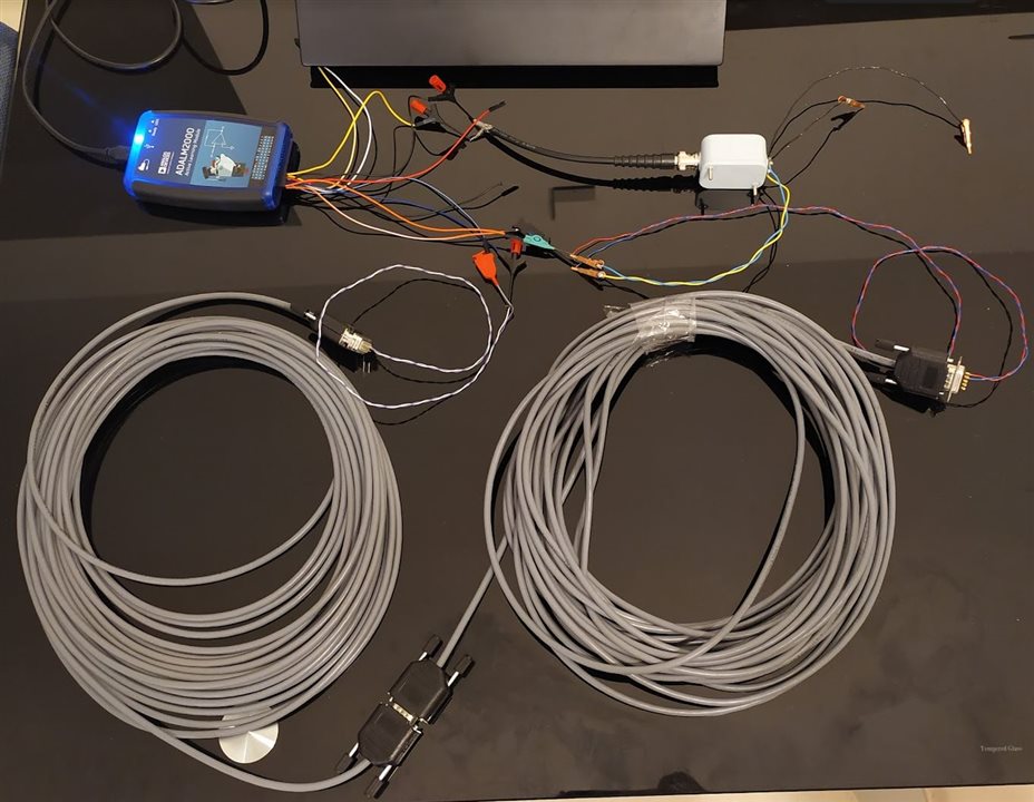
Here is how it all looks with the connections done, sitting on my dining table. 

Testing in Time domain

For the first test, the idea is to "launch" a signal into the cable and look at the signals at both ends of the DUT using ADALM2000's oscilloscope channels. 

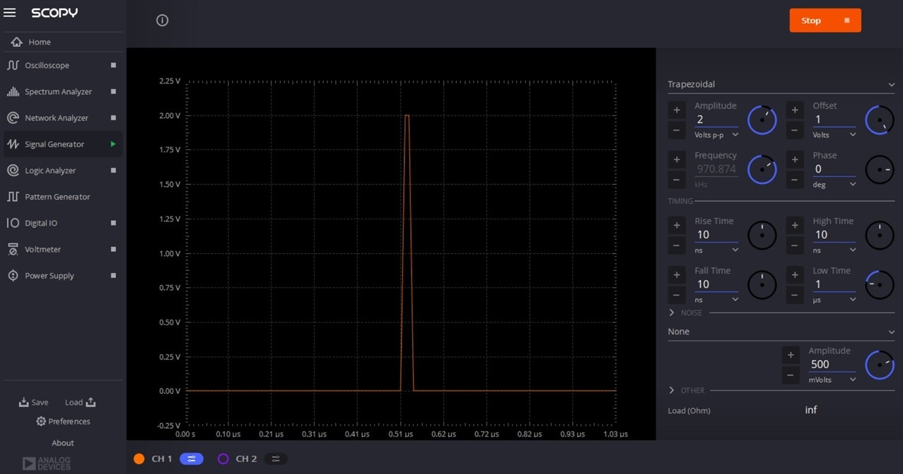
The most suitable test signal for this would be an impulse signal since it's easy to visualize and understand. Since there is no "pulse" waveform in the options, the best way to generate this using the ADALM2000's Function generator is to use the "Trapezoidal" waveform mode. This lets us choose the values of rise time, fall time, high time and low time independently, so we can build our own pulse.

I chose the smallest values for Rise time and Fall time that I could select, to give the most compact pulses. 1V was chosen as amplitude so that the signal is not too small, considering the ADC resolution, but also not too large, since slew rates are never infinite. When sending very fast signals/edges, it's generally good to keep the amplitudes low. This is why all high speed digital signalling use lower peak-to-peak voltages. The "high time" of pulse was chosen to keep the pulse compact, and the "low time" was chosen long enough so that any reflections would die down before the next pulse came in.

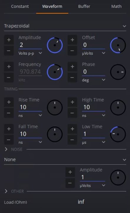
The scopy Signal Generator interface gives us a visual representation of what our signal would look like. This looks like an acceptable pulse to me.

Btw, I also found another way to generate a pulse, using the "Buffer" option inside the Signal Generator interface. Using it is very easy: First you create a sequence of values in Excel, save it as a .csv file and load it as a buffer inside Scopy. At this point you can set the sample rate and amplitude of the signal. Scopy shows a representation of the signal inside the GUI. Then hit "Start" when you are happy with the settings. In my case, the pulse I was able to generate using this option wasn't any different compared to the "trapezoidal" waveform described above so I'm not going to delve into it further. But just know that the option is there and is very easy to use.

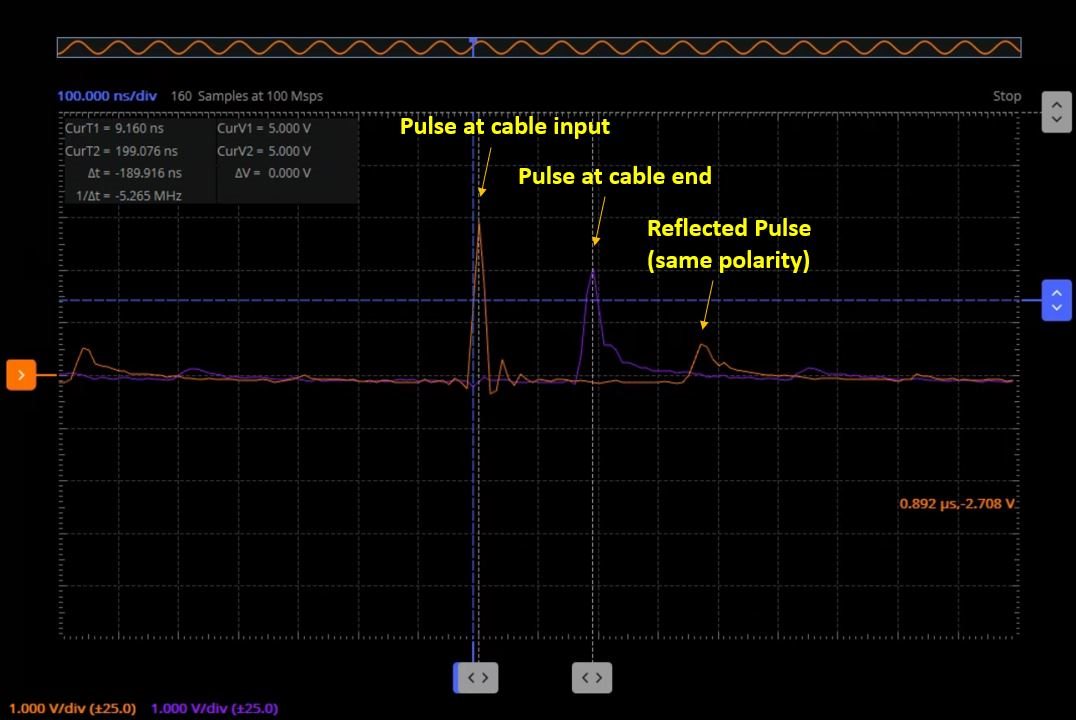
After setting the function generator to run continuously, I switched to the oscilloscope (inside ADALM200) to acquire the signals on the line. Trigger was used on Ch1. Here is the result:

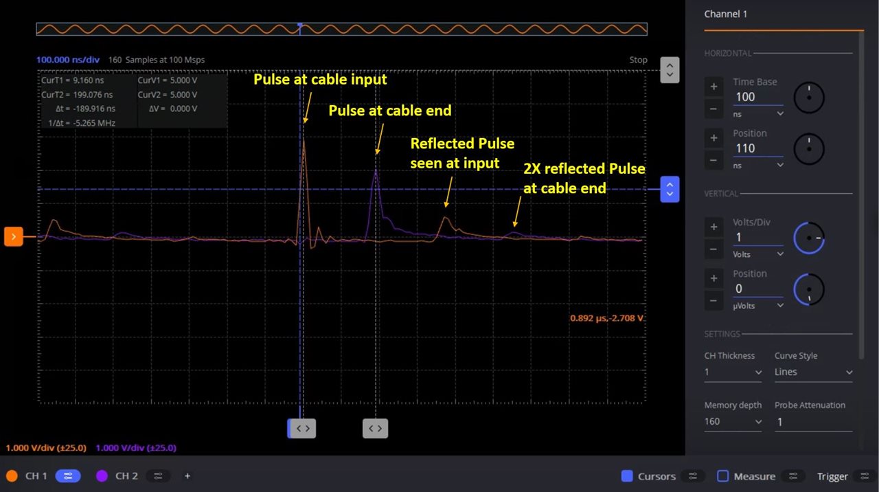
Interestingly, we can see the pulse travelling down the cable as a wave, going from one end to the other in ~190 nanoseconds! Afterwards, since the far end is unterminated, the pulse reflects back, just like a wave, and makes an appearance at the input side again. Yet again, it gets reflected from the input side and is seen at the output side after travelling the length of the cable 3 times. We see reflections after that also, but they become too small to observe.

Another Interesting thing I observe here is that the peaks are not as well defined as the pulse travels longer distances through the cable (and experiences reflections). One reason I can think of is that the "sharpness" of the pulse is from the higher frequency content in the pulse. We know well that the higher frequencies experience higher attenuation when passing through any medium compared to lower frequencies. So as the signals travels further and further, the signals has lesser of the high frequency energy, making the peaks appear less sharp. It helps to think about it in the frequency/fourier domain.

Note that the timebase is set to 100ns, which is the shortest timebase we can use for the ADALM2000. This is because of the sample rate limit on the ADALM2000 ADC. This also means that if I were using a cable smaller than this one (30m), it would get harder and harder to see these reflections due to successive pulses arriving within very short duration of each other. In other words, if you wanted to observe this phenomenon in an even shorter cable, you would need to use an oscilloscope with a higher sample rate, and possibly a faster pulse/edge generator also.

Since we know the length of cable (30m total - I measured it!), and now know the time it takes for the pulse to travel through the cable, we can calculate the Velocity of propagation for our cable:

V = S/t = 30m/182.35ns =  1.65 * 10^8 m/s

You might have noticed that I have used 182.35ns as time taken to travel 30m instead of 189.9 ns seen in the screenshot. This is because there is an uncertainty/error in every measurement. Since we're measuring small changes close to the sample rate limit of the device, to reduce error, instead of measuring interval between first two peaks, I measured the time interval between first and 4th peak, and divided it by 4 to get average time to travel 30m. This came out to 729.4ns / 4 =182.35ns average. 

I was expecting to get around 2 * 10^8 m/s (from searching the internet), however this is what we obtain experimentally. We are approximately 18% off. 

Initially I thought this is due to the extra length of the actual wires inside due to the twisting. To investiget this, I carefully measured and cut a 1m piece of this cable:

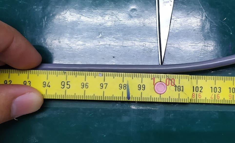
Then I stripped and removed the wires inside, straightened one wire as much as I could, and measured the straightened wire again.

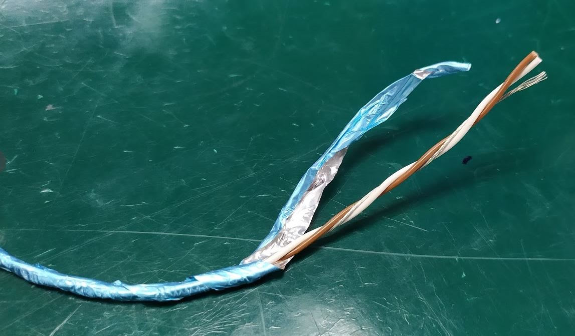
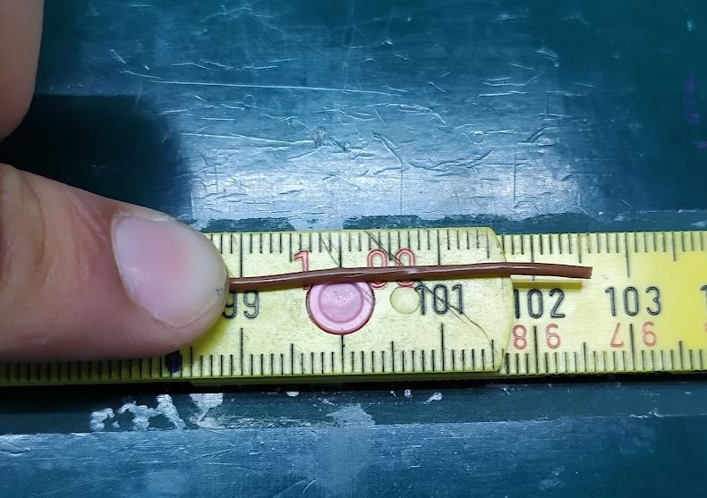
It was somewhat anticlimatic to find that the twisting was causing only ~3% increase in actual wire length. This still leaves us another ~15% of the travel time unaccounted for. 

I would love to hear any ideas/ possible explanations from the readers on this!

Testing in Frequency domain

Moving to the frequency domain, we will use the same setup/connections, but now investigate in the frequency domain. The spectrum analyzer does not yield much meaningful information based on my pulses, so I instead switch to my (now favourite) Network Analyzer inside the ADALM2000.

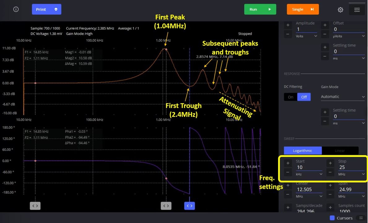
Since my BALUN's freq range is 10kHz to 60Mhz, and the ADALM2000's network analyzer works up to 25Mhz, I do my initial (logarithmic) sweep from 10kHz to 25MHz.

 Here we can make some very interesting observations.

The Amplitude response, which is a ratio of signal seen at Ch2 vs signal seen at Ch1, starts rising at frequencies above ~50kHz and shows a peak at 1.04Mhz. Afterwards it has a minima (trough) at 2.4Mhz, followed by more peaks and troughs, while the overall response seems to start to attenuate at higher frequencies.

So why are we getting this cyclic behaviour of peaks and troughs? 

Also, since we are seeing a ~10.8dB gain at the first peak, is the output signal getting bigger than even the input signal? How is that possible?

Using the "Buffer Previewer" function inside the Scopy software ("Network Analyzer" tab) we can "debug" this situation. As we move the buffer previewer cursor from left to right and look at the raw signals on both channels, we can see that it's not the output signal getting bigger but rather the input signal that is getting smaller! This results in increasing the Ch2/Ch1 ratio and we see it as a positive gain on the Amplitude graph.

To understand what's happening, recall two things:

1. The signal is travelling at a finite speed through the cable
2. The signal is getting reflected from the far end as we don't have the cable properly terminated into a matching load.

When the wavelength of the signal becomes short enough that a quarter of it becomes equal to the total lenth of the cable, the reflection at the far end makes the reflected signal out-of-phase with the signal we are sending from the input side. This causes a destructive interference on the input side. Thus our Ch1 observes a much smaller signal at that side. This is responsible for the increased Ch2/Ch1 ratio which we see as a positive gain on the Amplitude graph. The peak point is when the incident and reflected sinusoids line up exactly, giving the strongest destructive interference at Ch1. 

To illustrate this, I have drawn an illustration, shown below:

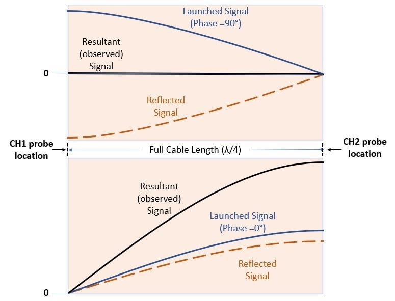
I have shown above the incident "wave" at 0 and 90 degrees phase. It can be seen that the signal at CH1 probe location is always zero irrespective of the phase of the incident wave. In reality the signal will not be completely zero, but rather a smaller signal due to the incident and reflected signals not being of same amplitude (hence imperfect destructive interference). This is what is known as a Standing Wave. I urge you to read the wikipedia article on standing waves to learn more. Btw, also notice that the maxima happen at phase difference of +/-90 and minima happen at 180 degree phase difference, which makes sense.

After the first peak, we have a trough/minima at ~2.4Mhz. The explanation is similar, except that this happens when the cable length is λ/2 (half of signal wavelength). The subsequent maxima and minima happen at odd,even multiples of these lengths and constitute the various "modes" of standing waves.

The other things that's apparent is how the response is reducing noticeably at higher frequencies. This shows that the higher frequencies are getting attenuated faster than the lower frequencies. This is the case for most cables. For signals at higher frequencies this is important to consider if choosing this cable for transmission.

Measuring cable's characteristic Impedance

We have observed that the electrical signals propagate like waves inside the cables/transmission lines. Each cable/transmission line has a "characteristic impedance) and anything that is connected downstream needs to match that characteristic impedance to prevent reflections and for the best signal energy transfer. But to match the characteristic impedance, first we need to know the characteristic impedance of the cable itself. 

We can do this by connecting a variable load resistor, and observing the reflections until we get no (or minimum) reflections back from the terminated end. At that moment, the values of the resistor is the characteristic impedance of the cable/transmission line. Let's try this with this cable.

The configuration is same as before, except that we have added a 200 Ohms multiturn potentiometer to the far end of the cable as a load. The value of 200 Ohms is chosen because typical characteristic impedances of twisted pair cables lie in the 80-130 Ohm range. Since the 200 Ohms potentiometer goes from 0-200 Ohms, it should cover the range nicely while giving us fine control on the value.

We return to our setup we used for our time domain experiments. Set the Signal generator to generate pulses, and observe the pulses at both sides of the cable again.

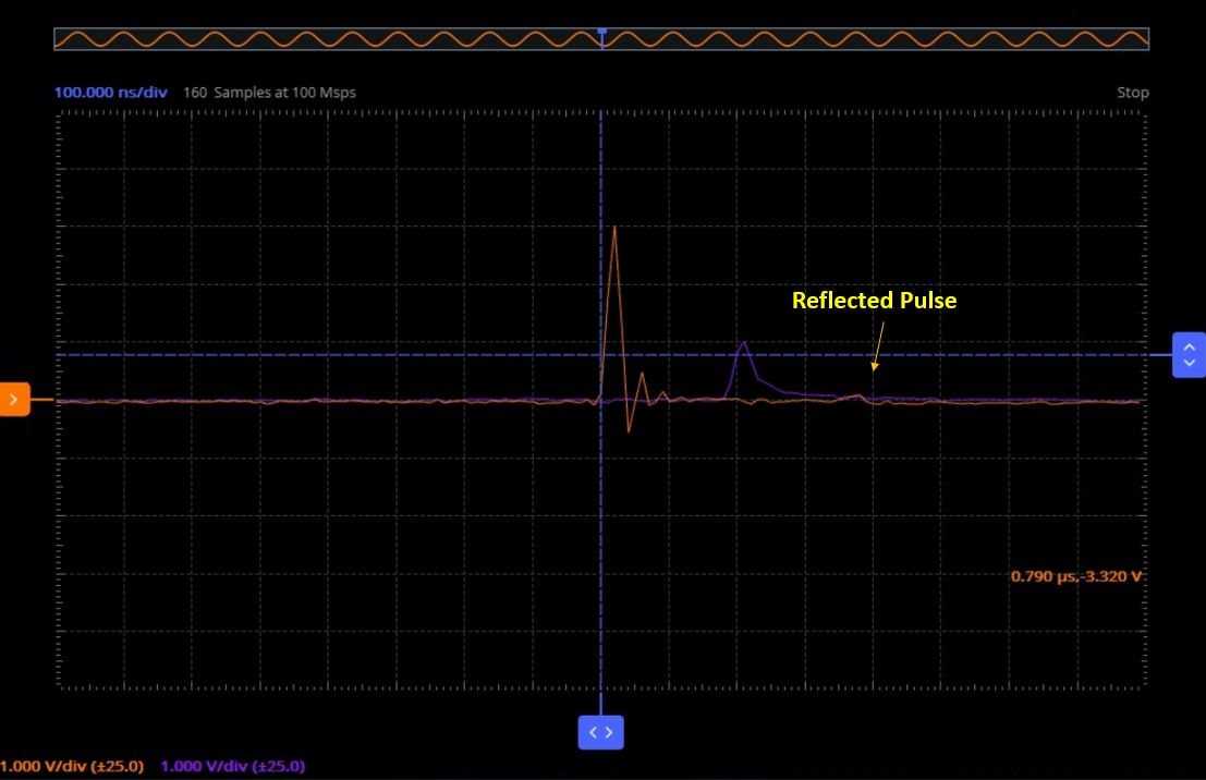
Previously, the far end of cable had no resistor connected, which can be considered as a resistor with very high value (infinity). In this case, we saw that the reflected pulse seen at input has same phase as the pulse we sent in. This confirms to the laws of physics, more specifically wave propagation/reflection, whereby the polarity of reflected wave stays same when a wave tries crossing from lower impedance medium to a medium with higher impedance. If we see this on the reflected pulse, we know we have set the resistor to a value too big.

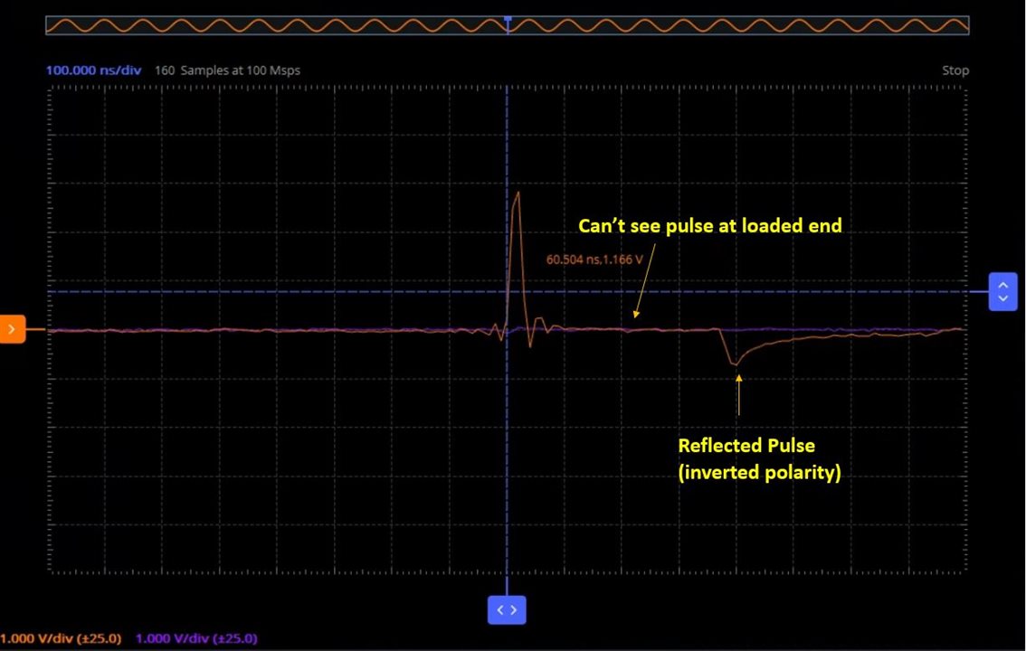
Now, if we go to the other extreme, i.e., if we load the far end with a resistor of very low value (or a "short"), the reflected wave inverts its polarity. This, again, confirms to the physics of wave reflections when interacting with a boundary to a lower impedance medium. If we see this on the reflected pulse, we know we have set the resistor to a value too small.

Finally, we can see what we get when the value of the load resistor is just right. We see the signal at the far end, but little or (ideally) no reflected pulse. In my case, this was the best I could tune my resistor to. This means that at this point the characteristic impedance of the cable matches the impedance of the load, and hence there are no reflections. This also means that maximum power is transferred from our input, via the cable, to the load, which is usually our goal.

At this point, we can also do a frequency sweep using the network analyzer to revisit the amplitude & phase responses. I have used the same sweep parameters and displaying with same limits as before to give a good comparison with the sweep we performed in our frequency domain experiments above. 

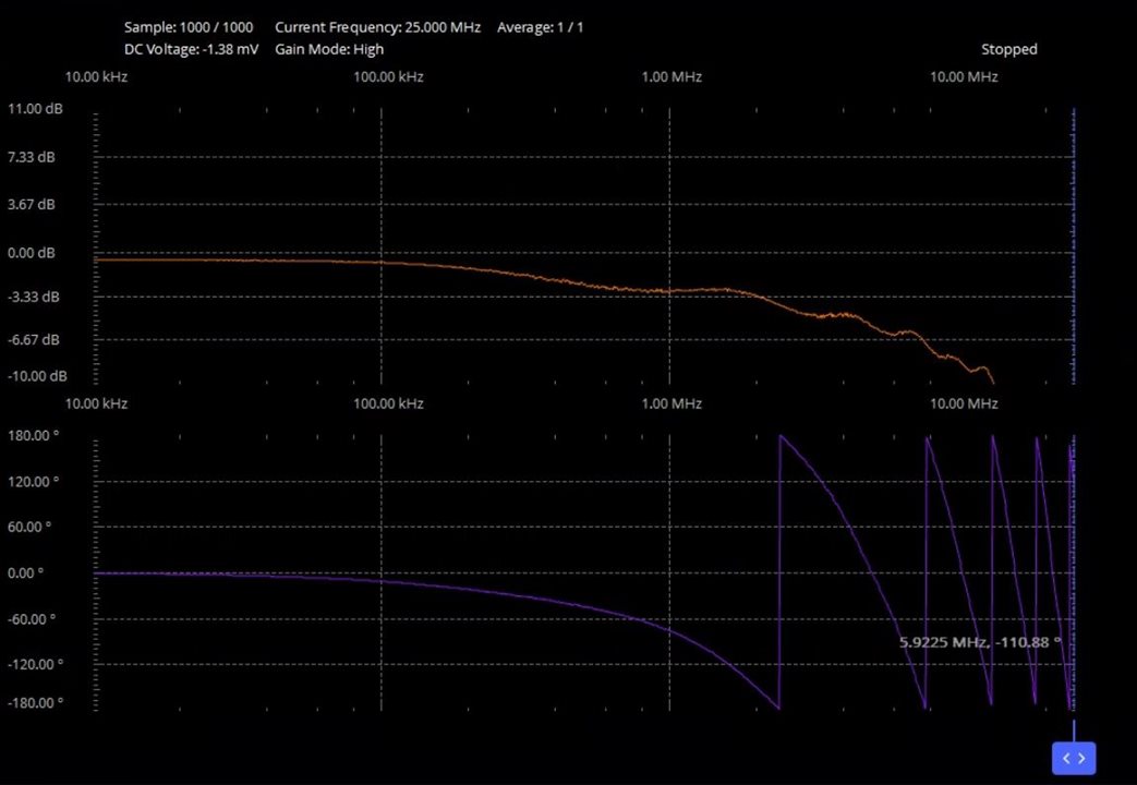
Here, we can see that our graph no longer starts at 0 db. This is expected since now we have a load at the other end which will load the signal at all frequencies (including DC). On the other hand, the peaks and troughs are not as pronounced as before. If we had a perfect termination we would not have seen any variation at all, but for this setup this is the best we can manage for now. We can also note that the higher attenuation at higher frequencies is still there, since our load can't change that characteristic of the cable.

Lastly, I took out the potentiometer and measured the actual value, which came out to be 80 Ohms. This means ~80 Ohms is the characteristic impedance of our cable.

Final words

That's it for these experiments with long cables/transmission lines. I learned a lot from these, and I hope you did too! A lot of the conclusions are based on my own (limited) understanding, so if you spot an error or want to add something, please do leave a comment!

Lastly, I have to say that it's quite amazing that I was able to do ALL of these interesting experiments in my home, on my dining table, thanks to the ADALM2000. If not for this device, the hassle of arranging the separate instruments and analyzing the results by other means would surely have prevented me from doing all of these experiments. And I think this is where the true value of an instrument like this lies!