


Why a neural network
Neural network is a subset of the machine learning universe. Machine learning refers to algorithms that can find patterns in numbers that represents a generic phenomenon. According to a wise software engineer at Google,
"If you can build a simple rule-bases system that doesn't require machine learning, do that"
However, if
- the problem can only be modelled with a long list of rules
- the environment is continually changing
- you need to discover patterns in a large collection of data
then machine learning is the tool to use.
In this project, I think that a threshold-based system (i.e. a system that generates an alert when acceleration rise above a fixed value) is not be reliable enough, if we consider the difficulty of distinguishing between some kind of falls and ordinary movements in elderly people’s life. A system that detects all falls but generates many false alarms make users unconfident about it.
Neural networks can be trained to "recognized" specific patterns in acceleration readings as "falls" and other patterns as "daily activities" by providing a sufficient set of examples, Furthermore, a neural network can make generalization, i.e. has the ability to correctly classify patterns that it has never seen before.
From a technical point of view, the best approach for detecting patterns in time series is a Recursive Neural Network (or RNN) and, more specifically, the implementation called Long Short Term Memory (or LSTM for short). Unlike feedforward neural networks, LSTM has feedback connections. It can non only process single data points (such as still images) but also an entire sequence of data (such as speech or video). For example, LSTM is applicable to task such as handwriting recognition, speech recognition and anomaly detection in network traffic or intrusion detection systems. A common LSTM unit is composed of a cell, an input gate, an output gate and a forget gate. The cell remembers values over arbitrary time intervals and the three gates regulate the flow of information into and out of the cell.
But, because
- the neural network is going to be run on a platform with limited hardware resources
- the neural network implementation I have chosen (TensorFlow Lite) only can run classification neural networks
I will try to implement the fall detection network using classification neural networks
The tools
I will use Tensorflow to model and train the neural network. This tool is very handy because it has an online version which requires no setup at all: you just need to open
https://colab.research.google.com/
and you can start tweaking your neural networks.
import tensorflow as tf
print(tf.__version__)
where I imported Tensorflow with alias "tf" and printed out Tensorflow version.
Modelling the neural network
Detecting a fall is a typical classification problem, in that we want to predict whether "something" belongs to a class or another. This means we are taking accelerometer data as input and we are generating a binary output: 0 if the input data is classified as "daily activity" or 1 if the data is detected as a "fall".
A more precise classification is possible. For example, I could have trained the network to label each pattern as "walking", "walking downstairs", "walking upstairs" but, considering that
- I am interested in detecting falls as precisely as possible
- Labelling is more reliable if the set of possible labels is small
- we want a lightweight neural network to save memory and CPU time on the Arduino Nano
I opted for the binary classification I mentioned before.
Actually, because we are analysing a time serie, it would have been better to use something like LSTM (Long Short Term Memory) networks, but TensorFlow Lite includes a limited set of operators, (available operators are listed here), I also found that there is a docker image with all the tools required to cross-compile TensorFlow Lite for any ARM platform. May be I will give it a try...
With all this prerequisites in mind, the Multilayer perceptron (MLP) should be considered the best solution for pattern classification. Technically, these are feedforward neural networks trained with the standard backpropagation algorithm. MLP are networks that learn how to transform input data into a desired response. With one or two hidden layers, they can approximate virtually any input-output map.
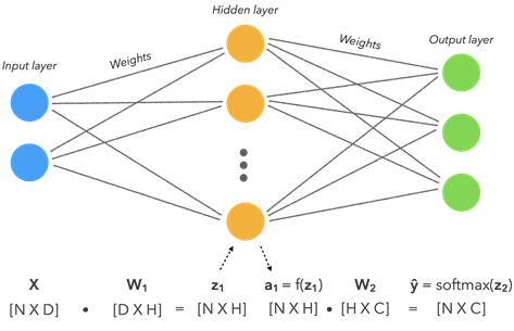
Architecture of a binary classification neural network
I'am not going to cover all the details about neural network here, since there are many resources on the Internet that covers the topic in great details. My favorite resources are
In general, a neural network is made of
- an input layers
- some hidden layers
- An output layer
Values are provided to the input layer, multiplied by values called weights and propagated to the next layer. Weighs can be adjusted so that the output for a given input matches the expected output by means of an algorithm called optimizer. The most commonly-used optimizers are SGD (Stochastic Gradien Descent) and Adam. To measure of how good the value predicted by the neural network matches the expected output, we can select a proper loss function. For regression problem, the typical loss functions are MAE (Mean absolute error) or MSE (Mean squared function). For classification problems, Cross entropy is the most commonly used
As per Hands-On Machine Learning with Scikit-Learn, Keras & TensorFlow Book by Aurélien Géron, the following are the standard values you'll often use in a classification neural network
| Hyperparameter | Typical value for binary classification problems |
|---|---|
| Input layer shape | Same as number of features |
| Hidden layers | Problem specific |
| Neurons per hidden layers | Problem specific, generally from 10 to 100 |
| Output layer shape | 1 |
| Hidden activation | Usually ReLU (Rectified Linear Unit) |
| Output activation | Sigmoid |
| Loss function | Cross entropy |
| Optimizer | SGD (Stochastic Gradien Descent), Adam |
As I said, the input of the neural network are the accelerometer readings. Since we have 6 readings (3 linear accelerations and 3 angular accelerations) and we need to feed the network with readings over a given time window, the input will be a matrix of
n samples x 6 readings
The number of samples "n" needs to be selected accurately, because there are several constraints to take into account
- the sensor readings have to be stored in the Arduino RAM, which is limited to 32 kb
- as a rule of thumb, the more data we feed into the neural network, the more precise will be the classification
- the more frequently we sample data, the more precise will be the classification
- the longer we sample data, the more precise will be the classification
With these considerations in mind, and considering that most of the work in fall detection algorithms use a 50Hz sampling rate and an event duration of 12 - 15 seconds, we will take
n = 300
This value will eventually be decreased should the available RAM be insufficient to run the neural network.
So this is the diagram of how our neural network will work
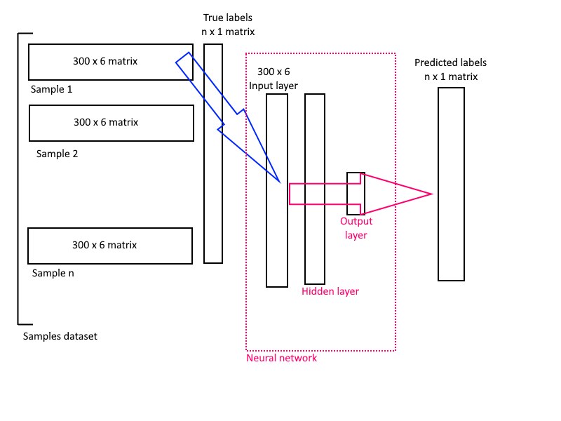
Neural network is fed with all the samples in the dataset, label is predicted and compared with the expected label. During training phase, comparing predicted output with the expected output makes it possible to adjust the weights of the neural network's internal connections
Training data
As MLPs are supervised, they require a set of known patterns with known responses to get trained. With one or two hidden layers, they can approximate virtually any input-output map. Sistemic provides a very interesting dataset.
This dataset was generated with collaboration of 38 volunteers divided into two groups: elderly people and young adults. Elderly people group was formed by 15 participants (8 male and 7 female), and the young adults group was formed by 23 participants (11 male and 12 female). Each person has performed different activities. Accelerometer and gyroscope data has been sampled at 200Hz and saved in text files with 9 columns:
- 1st column is the acceleration data in the X axis measured by the sensor ADXL345.
- 2nd column is the acceleration data in the Y axis measured by the sensor ADXL345.
- 3rd column is the acceleration data in the Z axis measured by the sensor ADXL345.
- 4th column is the rotation data in the X axis measured by the sensor ITG3200.
- 5th column is the rotation data in the Y axis measured by the sensor ITG3200.
- 6th column is the rotation data in the Z axis measured by the sensor ITG3200.
- 7th column is the acceleration data in the X axis measured by the sensor MMA8451Q.
- 8th column is the acceleration data in the Y axis measured by the sensor MMA8451Q.
- 9th column is the acceleration data in the Z axis measured by the sensor MMA8451Q.
Data in the files is the raw ADC reading. To convert raw data to acceleration, we can apply this formula
Acceleration [g]: [(2*Range)/(2^Resolution)]*AD
For the angular velocity read by the gyroscope, the formula is
Angular velocity [°/s]: [(2*Range)/(2^Resolution)]*RD
Ranges and resolutions of the sensors are the following
| Sensor | ADXL345 | ITG3200 | MMA8451Q |
|---|---|---|---|
| Resolution | 13 bits | 16 bits | 14 bits |
| Range | +- 16g | +-200 °/s | +- 8g |
Preprocessing
In order to be used in this project, I created a simple application in C# that takes the text files in the dataset and performs the following preprocessing operations
- gets data related to ITG3200 and MMA8415Q sensors
- downsamples from 200Hz to 50Hz
- starts saving data to output final one second before the acceleration norm or the angular velocity reaches a threshold value
- limits the number of samples in each file to 300
- converts data [g] and [°/s]
- saves data to a file whose name has the format
<ACT>_<PROGR>.csv
where
<ACT> is the code of either an activity or a fall as listed in the Readme file included in the Sistemic dataset
<PROGR> is a progressive number
The reason I applied a peak detection algorithm to the samples in the Sistemic dataset is to train the neural network with a set of time series that resembles as close as possible the real data collected by the Arduino Nano 33 IoT board, where the peak detection algorithm will be implemented. A peak detection algorithm is required because the wearable device will collect data continuously and it practically unfeasible to invoke the neural network every time a sample is read from the accelerometer because:
- invoking the neural networks takes for sure an amount of time larger than the accelerometer sample time. A minimum sample frequency of 50 Hz (i.e. a sample every 20 ms) is required in order to be able to reliably analyze time serie
- storing a complete window would take a lot of RAM, which is the scarcest resource in this challenge
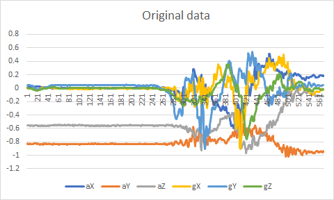
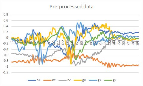
Here is an example of the original time series from the dataset (on the left) and the time series saved in the csv used to train the neural network (on the right).
Files generated by the application have been uploaded to my Google Drive in order to be loaded by the Python code I will write in TensorFlow

Creating tensors
Next step is to create tensors from the csv files. Tensors are matrixes optimized for execution on a TPU (Tensor processing unit), that is to say a special piece of hardware developed by Google to run Machine Learning algorithm. For more details about what a tensor is, I think this video is very useful.
Splitting the dataset
Last step in preparing our dataset is to split all the available inputs in two sets
- Training set: the model will learn from this data, which is typically 70-80% of the total data available
- Test set: the model will be evaluated on this data to test how good was to learning process
Some sources mention a third dataset (which I am not going to use)
- Validation set: this is data the model will get tuned on
To split the dataset, there is a very handy function in the scikit-learn package: train_test_split
# Split dataset in training and test sets
from sklearn.model_selection import train_test_split
X_train, X_test, y_train, y_test = train_test_split(X,
     y,
     test_size=0.2,
     random_state=1337) # set random state for reproducibility
Normalization
A common practice when working with neural networks is to make sure all of the data is in the range 0 to 1. This process is called normalization. Since this is done by subtracting the minimum value than dividing by the maximum value minus the minimum value, this process is also called min-max scaling. There are lot of information about the best practices in data preprocessing on scikit-learn website.
This is the code to normalize our data
from sklearn.compose import make_column_transformer
from sklearn.preprocessing import MinMaxScaler

# Create a column transforme
ct = make_column_transformer(
     (MinMaxScaler(), ["ax", "ay", "az", "gx", "gy", "gz"])
)

# fit column transformer on the training data only (doing so on test data would result in data leakage)
ct.fit(X_train)

# transform training and test data with normalization
X_train_normal = ct.transform(X_train)
X_test_normal = ct.transform(X_test)
Building the neural network
It's time to build the neural network. In Tensorflow, the process is
- Create the model
- Compile
- Train
- Evaluate
- Tweak the model and return to step 2
Creating the model
Creating a model in Tensorflow is very easy
# set seed for reproducibility
tf.random.set_seed(2309)

# create the model
model = tf.keras.Sequential([
     tf.keras.layers.Dense(4, activation=tf.keras.activation.relu),
     tf.keras.layers.Dense(4, activation=tf.keras.activation.relu),
     tf.keras.layers.Dense(1, activation=tf.keras.activation.sigmoid),
])
This model as 2 hidden layers with a relu activation function and an output layer with 1 single node and a sigmoid activation function. The shape of the output node is 1 because we need just one single output value (fall / not fall). The number of hidden layers and the number of nodes in each layer has to be tuned according to the specific problem.
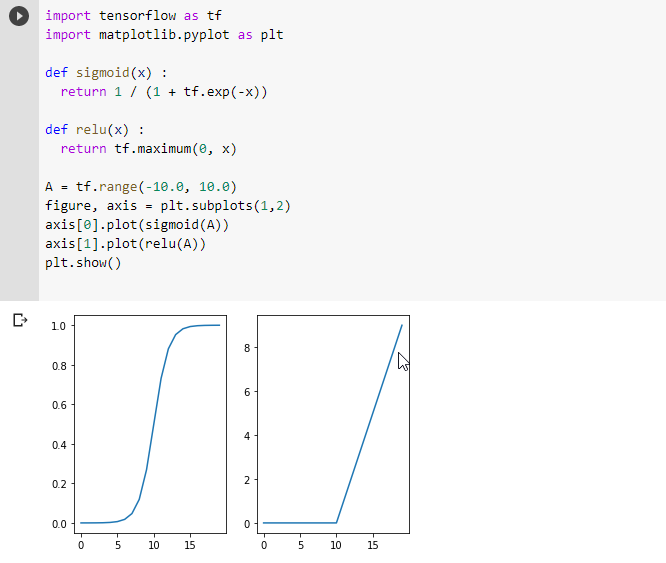
One of the first questions I was asking myself when I started studying neural networks was: how they can find patterns in inputs? A classification should lead to identify an n-dimensional contour surface to separate one class from another, but you need some non-linear correlation between inputs and outputs. Now I know the answer lies in the activation functions. Both relu and sigmoid activation functions are non linear (see plots below). This allow the network to approximate any non-linear correlation between inputs and outputs
Compiling the model
The model needs now to be compiled
# build the model
model.compile(loss=tf.keras.losses.binary_crossentropy,
     optimizer=tf.keras.optimizers.Adam(),
     metrics=['binary_accuracy']
);
The metrics is the method the measure the predicted output when compared to the expected output. Here we used binary_accuracy, because we are creating a model for binary classification. Another possible metric could be 'accuracy', which is a special metric in Keras because it can be used in any kind of regression or classification problem.
In a binary classification problem, there are some other metrics that are of interest to us
| Metric | Definition | Code |
|---|---|---|
| Accuracy | Percentage of correct predictions. For example, 95% accuracy means that 95 predictions out of 100 are correct
| sklearn.metrics.accuracy.score() tf.keras.metrics.Accuracy() |
| Precision | Proportion of true positives over total number of samples. Higher precision leads to less false positives (i.e. model predicts 1 when it should have been 0)
| sklearn.metrics.precision.score() tf.keras.metrics.Precision() |
| Recall | Proportion of true positives over total number of true positives and false negatives (i.e. model predicts 0 when it should have been 1)
| sklearn.metrics.recall.score() tf.keras.metrics.Recall() |
| F1-score | Combines precision and recall into one metric
| sklearn.metrics.f1_score() |
| Confusion matrix | Represents in a 2D matrix the number of predicted class by the model vs the expected class | |
| Classification report | Collection of some the main classification metrics, such as precision, recall and f1-score | sklearn.metrics.classification_report() |
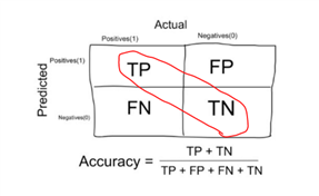
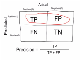
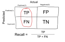
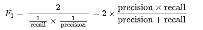
(images from https://anarinsk.github.io/lostineconomics-v2-1/machine-learning/basics/2020/04/19/classification-metrics.html )
Because we want to avoid false positive (i.e. falls that are detected are activities of daily life), our goal is to optimize the precision
Training the model
Finally we can train the model with our training dataset
# train the model
hist = model.fit(X_train_normal, y_train, epochs=100, verbose=0)
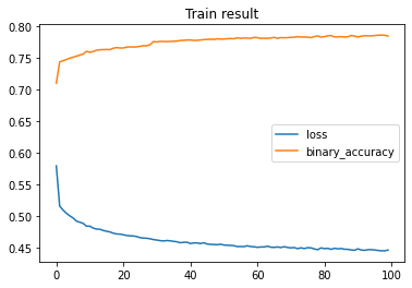
The first version of the model provided these results
Accuracy is less the 75%. Some serious improvements to the model are required!
Model improving process
The common ways to improve the model is to
- add new layers: adding new layers, however, makes the neural network that is more prone to memorization than generalization
- increase the number of hidden units
- change the activation functions
- change the learning rate: every optimizer works by selecting the weight that looks most promising (i.e. the weight that, if changed, will bring the model closer to the expected output) and changes the value to an amount equal to the learning rate. This means that
- if the learning rate is too small, the training process will be extremely slow and will require a consistent amount of time to reach the optimal solution
- if the learning rate is too large, the optimizer will "jump" around the optimal solution without reaching it
- fitting on more data: this means to collect more samples
- fitting for longer: this is the number of iterations the learning process will do to adjust the weights of the connections among the neural network's nodes. (see the "epochs" parameter of the fit() method). There is a limit where the loss function will reach a plateau and there is no sense in increasing the number of epochs further. In this cases, it's better to increase the number of layers or hidden units to make the neural network fit a more complex surface
We immediately see in the chart is the that binary_accuracy flattens after a very limited number of iterations. This is a symptom of a model that is too simple for the phenomenon we are trying to predict. So the first thing is to increase the number of nodes in the hidden layers and/or add new layers. As a dummy in neural networks, I don't have the experience to find the most convenient optimization path. I just followed a trial-and-error process to find out which are the sets of parameters that are best suited for my specific problem. Hopefully I will discover a more systematic approach in the near future...
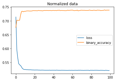
But with 100 nodes this is what happened
No improvements or very marginal improvements. Looks like the input data can not be mapped to expected results reliably using the multilayer perceptron. At this point, I tried a feature-based different approach (more about this later). I will now talk a little bit about how to determine the best learning rate because this optimization procedure will also be used for the second approach I experimented with
To understand how well the model is learning, we can plot the loss curves, i.e. how quickly the "distance" between predicted outcome and expected outcome decreases. The fit() method of the model returns an object whose history property stores the value of loss function for each iteration. We can plot easily plot such values using pandas library
import pandas as pd
hist = model.fit(X_test, y_test)
pd.DataFrame(hist.history).plot()
Finding the best learning rate
To find the best learning rate, we can plot a graph of learning rates against losses. First, we need to set a learning rate scheduler callback
# Create a learning rate scheduler callback
lr_scheduler = tf.keras.callbacks.LearningRateScheduler(lambda epoch: 1e-4 * 10**(epoch/20)) # traverse a set of learning rate values starting from 1e-4, increasing by 10**(epoch/20) every epoch

# Fit the model (passing the lr_scheduler callback)
hist = model.fit(X_train,
  y_train,
  epochs=100,
  callbacks=[lr_scheduler])
# Checkout the history
pd.DataFrame(history.history).plot(figsize=(10,7), xlabel="epochs");
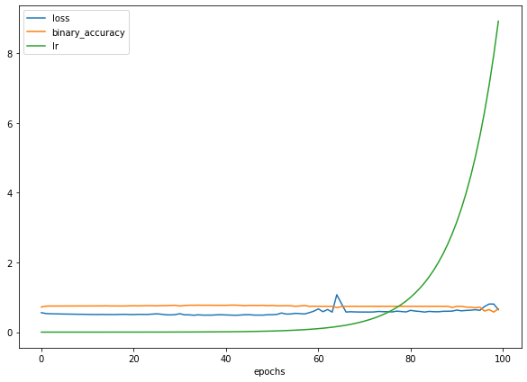
To find out the optimal value, we can plot loss versus the learning rate
# plot the learning rate versur the loss
lrs = 1e-4 * (10 ** np.arange(100)/20))
plt.figure(figsize=10,7))
plt.semilogx(lrs, hist.history(["loss"])
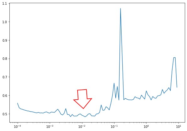
The rule of thumb is to take the learning rate value where the loss is still decreasing but not quite flattened
Other metrics
Keras does not include metrics like precision, recall or F1-score, but all these metrics can be easily checked with just a few lines of code by running the metrics provided by the Scikit-learn API.
Evaluating the model
We can evaluate how the model is good at predicting the expected outcome on the test dataset. The most relevant metrics have already been introduced. The following code calculates and prints out precision, recall, F1-score and AUC
# evaluate the model
train_acc, train_loss = model.evaluate(fX_train, y_train, verbose=0)
test_acc, test_loss = model.evaluate(fX_test, y_test, verbose=0)

print('Loss - Train: %.3f, Test: %.3f' % (train_loss, test_loss))

# compute precision, recall, F1-score
from sklearn.metrics import precision_recall_curve
from sklearn.metrics import f1_score
from sklearn.metrics import auc
import seaborn as sns

y_predict = model.predict(fX_test)
y_predict_labels = np.round(y_predict)
precision, recall, thresholds = precision_recall_curve(y_test, y_predict_labels)
f1 = f1_score(y_test, y_predict_labels)
auc = auc(recall, precision)
print("Precision: ", precision[1])
print("Recall: ", recall[1])
print("F1-score: ", f1)
print("AUC: ", auc)
One step back: features extraction
After the first experiment, I realized that time series can not be ingested in the neural network. There are so many inputs (300 samples for each of the 6 IMU DOFs) that the network can be trained to generated the expected data reliably or may be there are some many inputs that neural network can not determine what is relevant. So I tried to identify a certain number of features that can "summarize" the input data from sensor and make the machine learning process work better and faster. This process is called features selection. There are many different feature selection methods, and all of them are intended to reduce the number of input variables to those that are believed to be most useful to a model in order to predict the target variable. This diagram is very handy to select the correct feature selection method

Since the fall detection problem is a classification predictive modeling problem with numerical input values, we can select between two methods (both of them are correlation based)
- ANOVA correlation coefficient (linear, implemented in scikit-learn by the f_classif function)
- Kendall's rank coefficient (nonlinear)
I started from a long list of possible aggregation functions to apply to the IMU readings and that, in my opinion, may contain a good indication of a fall event was occurred. The initial list of aggregator included
- minimum
- maximum
- average
- standard deviation
- median
- skew
- magnitude
- slope
- absolute minimum
- absolute maximum
and many others. From this initial lists, I applied a top-k selector to determine which features have more correlation with the output
import numpy as np
import matplotlib.pyplot as plt
from sklearn.feature_selection import SelectKBest, f_classif

# check which are the most promising
featuresselector = SelectKBest(f_classif, k=2)
selector.fit(fX_train, y_train)
scores = np.where(selector.pvalues_ != 0, -np.log10(selector.pvalues_), 0)
scores /= scores.max()

fX_indices = np.arange(fX.shape[-1])
labels = ['avgaX', 'avgaY', 'avgaZ', 'stdaX', 'stdaY', 'stdaZ', 'adcaX', 'adcaY', 'adcaZ', 'minaX', 'minaY', 'minaZ', 'maxaX', 'maxaY', 'maxaZ', 'avgAcc','avggX', 'avggY', 'avggZ', 'stdgX', 'stdgY', 'stdgZ', 'adcgX', 'adcgY', 'adcgZ', 'mingX', 'mingY', 'mingZ', 'maxgX', 'maxgY', 'maxgZ' , 'avggAcc']
x = np.arange(len(labels))
indices = scores.argsort()[-16:][::-1]
print(list(np.array(labels)[indices]))
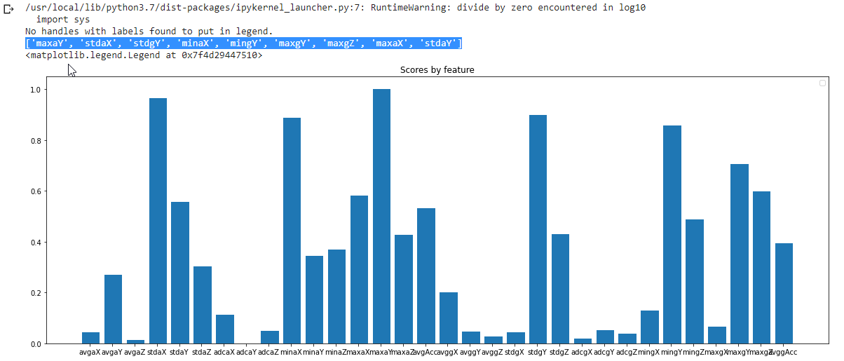
I tested with the a different number of the most representative features and I found that the best results comes with a set of 32 features, which, luckily, are also easy to compute!
I fed the neural network with a set of the 32-features input data extracted from the original dataset and the results are very encouraging. Here are the metrics calculated with a multilayer perceptron with different number of nodes in the hidden layer
| Number of nodes | Result |
|---|---|
| 10 nodes | 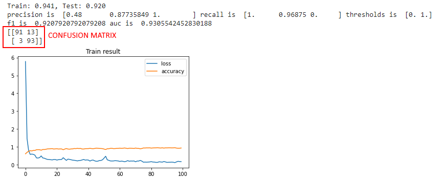 |
| 25 nodes | 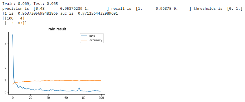 |
| 50 nodes | 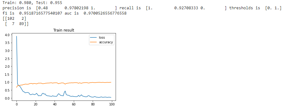 |
| 75 nodes | 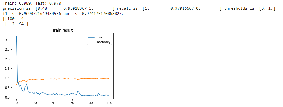 |
With 75 nodes, results are getting slightly worst, so somewhere between 50 and 75 nodes there is the optimum number of nodes for this problem. I tried to add some extra hidden layers, but I didn't see any improvement in the F1 score, so I will keep a neural network with a single hidden layer with 50 nodes the optimal solution for the fall detection problem
Converting the model
After the model has been properly tuned, it can be exported to a Tensorflow Lite model
# Setup environemnt
!apt-get -qq install xxd

# convert the model to the Tensorflow Lite format without quantization
converter = tf.lite.TFLiteConverter.from_keras_model(model)
tflite_model = converter.convert()
open("ace_model.tflite", "wb").write(tflite_model)
!echo "const unsigned char model[] = {" > /content/model.h
!cat ace_model.tflite | xxd -i >> /content/model.h
!echo "};" >> /content/model.h
(please note that there is an error in the tutorial Tensorflow notebook here: there is an "echo <model>.tflite" instead of "cat <model>.tflite")
The generated file (model.h) can now be downloaded and copied into the same folder as the Arduino sketch
The final model.h is about 50 kbytes in size. The first thing to do before proceeding further with the project is to test if it fits in the Flash and RAM of Arduino Nano 33 IoT. For this reason, I created a quick-and-dirty application where I included all the libraries I'am going to need to complete my project (namely WiFiNINA, ArduinoBLE, LMS6SD3, TensorflowLite) and some static buffers where I will collect the IMU sensor data. The compiler summary is quite reassuring: I think I can fit all the application inside the microcontroller!

Source code
Here are the TensorFlow notebooks I created to build the neural network of this project
https://colab.research.google.com/drive/1Ww_Zza3sXLLMNdnrUTgDkbKlw9mpZp34#scrollTo=W8jE-BZfZtz7
https://colab.research.google.com/drive/1_lLyAVyToVh_kdUaVrxRozjhyjySnow5#scrollTo=PFGZQZUK-AUI
| Previous post | Source code | Next post |
|---|---|---|
| ACE - Blog #3 - Sending notifications | https://github.com/ambrogio-galbusera/ace2.git | ACE - Blog #5 - Sensing the world |
Top Comments