


In my last blog posting, I tried to characterise the accuracy and noise performance of the Mikroe Current 6 Click incorporating the Analog Devices MAX40080 Precision, Fast Sample-Rate Digital Current Sense Amplifier using an SMU and PSU, but instead got some unexpected results. A 3-4Hz “dip” was appearing in the current data which caused a significant amount of noise to be registered on the readings, even though “on-the-whole” the average results seemed correct. This did not affect voltage data and suggested this is not an issue with the code but is part of the way the unit was working.
I was not satisfied with this result. It didn’t look right and I knew that it shouldn’t behave like this. To try and disentangle the cause, I proceeded with what I considered the best course of action – working a different platform to see if anything changed.
Table of Contents
Can I Get a Speed Check? Arduino MKR WiFi 1010 Enters the Ring
The easiest way to debug the issue of the mystery dips and to try and catch higher sample rates was just to try the Click on a different platform entirely. Rummaging around, I found a few traditional 8-bit AVR Arduinos, but I thought they’d be too slow, so I settled on an Arduino MKR WiFi 1010 that I previously received as part of an Omron Environmental Sensors RoadTest. It is a 32-bit, 3.3V-based board with native USB-CDC interface, which I thought would be ideal.
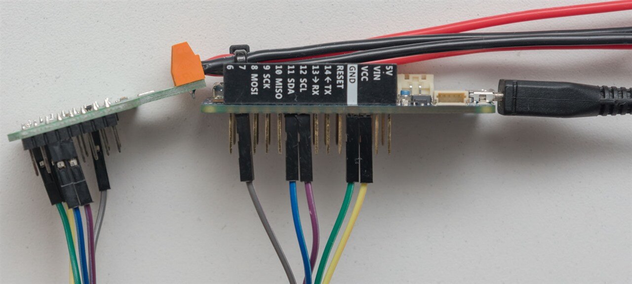
Thankfully, Click boards use traditional 2.54mm header pins, so I could just use a short segment of Dupont jumper wire to connect it to the pins on the MKR. In this case, power, ground, SCL and SDA were obvious, while I chose to use Pin 7 for the Enable signal. The Alert interrupt line was not connected as I am not using it, and the 5V line was not connected as it is only used for the 5V I/O level translation assuming you have moved the jumper on the board to enable it.
I started by porting my whole code over to the MKR which was easy enough … but I soon discovered nothing worked. As it turns out, running the I2C bus at 1MHz on the MKR just didn’t work – perhaps the Dupont wire was a stretch too far, but 900kHz worked fine so I settled for that. Already, the MKR was at a disadvantage compared to the Raspberry Pi.
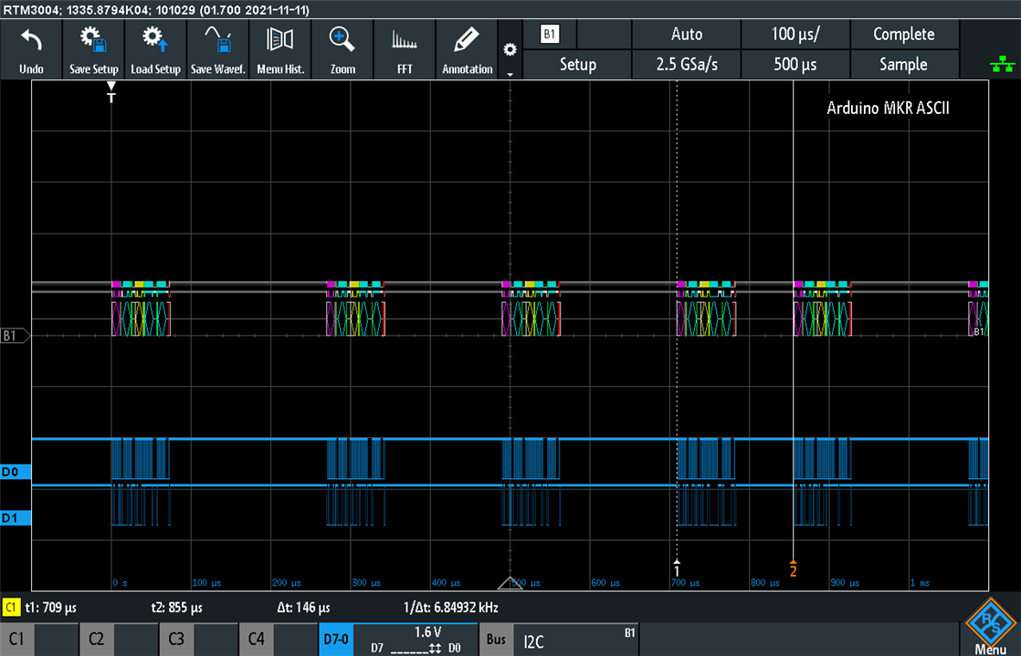
Unfortunately, the performance was disappointing. Whereas I was easily reaching ~12kHz on the Raspberry Pi, the MKR was putting out closer to 4.5kSa/s on a sustained basis, with the inter-query time varying depending on the data and the transformations necessary to turn it into an ASCII value and then push that to the PC. This was not unexpected, I suppose, because the microcontroller isn’t particularly powerful.
As a result, I decided to make the job for the MKR much easier – now its job is just to read two bytes from the FIFO, decide if they are valid by checking one bit, and if so then write both bytes out on the USB-CDC emulated serial. The code was as follows:
#include <Wire.h>
#define ADDR 0x21
#define CLKR 900000

void write24 (uint8_t addr, uint8_t reg, uint8_t by0, uint8_t by1, uint8_t by2) {
  Wire.beginTransmission(addr);
  Wire.write(reg);
  Wire.write(by0);
  Wire.write(by1);
  Wire.write(by2);
  Wire.endTransmission();
}

void write16 (uint8_t addr, uint8_t reg, uint8_t by0, uint8_t by1) {
  Wire.beginTransmission(addr);
  Wire.write(reg);
  Wire.write(by0);
  Wire.write(by1);
  Wire.endTransmission();
}

void setup() {
  Serial.begin(921600);
  while (!Serial) {
  }
  pinMode(7,OUTPUT);
  digitalWrite(7,HIGH); // Enable Click
  delay(250); // Power-up delay
  Wire.begin();
  Wire.setClock(CLKR); // 1MHz FM+ Mode
  write24(ADDR,0x00,0x00,0x00,0xB7);
  write16(ADDR,0x0A,0x00,0xB4);
  write16(ADDR,0x00,0x03,0x0F); //XX,5E 1MSa/s + 128 avg
                                //XX,0F 512Sa/s + 0 avg
                                //03,XX - Range 5A,
                                //43,XX - Range 1A
  write16(ADDR,0x0A,0x00,0x34);
}

void loop() {
  Wire.beginTransmission(ADDR);
  Wire.write(0x0C);
  Wire.endTransmission(false);
  Wire.requestFrom(ADDR,2,true);
  uint8_t lsb = Wire.read();
  uint8_t msb = Wire.read();
  if (msb & 0x80) {
    Serial.write(msb);
    Serial.write(lsb);
  }
}
On the PC side, I would use a Python program to read those bytes (it is lazy, so it doesn’t care about alignment, but the alignment is guaranteed on the first start) and perform the scaling computations and logging. The code on the PC looks like this:
import serial
import time

ser = serial.Serial("COM41",921600)

f = open("datafile"+str(time.time())+".csv","a")

i = 0

while i < 1000000 :
  fifod = ser.read(2)
  val = (fifod[0] << 8) | fifod[1]
  dsign = val & 0x00001000
  dvalue = val & 0x00000FFF
  if dsign != 0 :
    dvalue = dvalue - 4096
  f.write(str(time.time())+","+str(dvalue)+"\n")
  i=i+1
It was then I discovered the harsh truth …
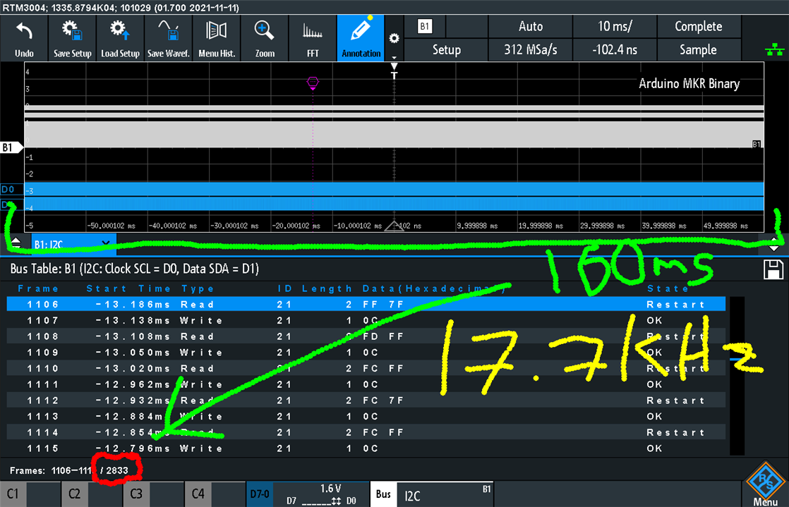
With the unit operating but the virtual CDC port closed, we were seeing a nice sample rate of about 17.7kHz.
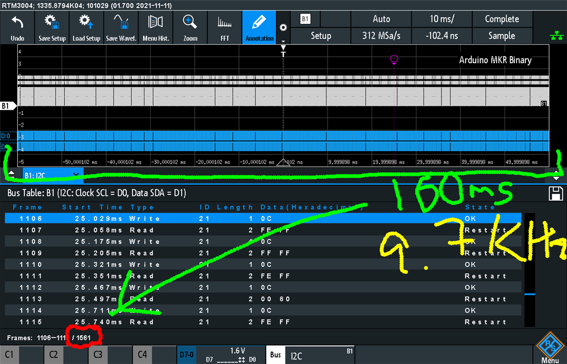
But once the CDC port was opened, the rate was now just 9.7kHz and in practice, varied quite a bit. This again meant that despite dividing the tasks, a meaningful increase in speed was not achieved simply because of the overhead of dealing with the data. Perhaps going back to the Raspberry Pi and using C may help a bit, but perhaps the best solution would be to go FPGA-based.
Scrap the Speed – What About the Readings?
I borrowed the above code but changed the sample rate to the leisurely 500Sa/s setting to see what the noise measurements would look like given this set-up. Would it be spiky, or would it be clean?
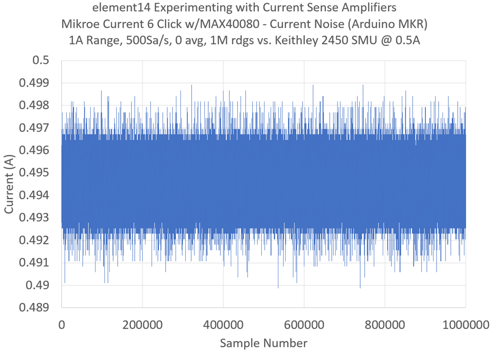
As it turns out at 1A … it was clean.

It was even bell-shaped in its distribution which was the right result. What gives? The code was pretty much a direct port. Was it a matter of range?
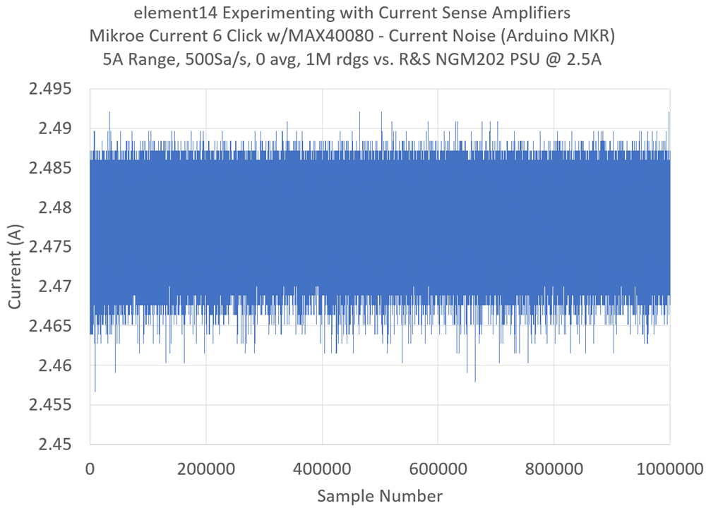
Nope! The 5A range was also decidedly clean …

… although slightly less bell-shaped because of shunt heating it would seem. This result was a definitive one though – the MAX40080 was not to blame! It should also prove to be a big hint to me as to the cause …
Power and Signal Integrity on the Raspberry Pi?
This had me wondering … what does the power on the Raspberry Pi look like? While the MAX40080 does sport fairly impressive power supply rejection ratios in its datasheet, poor quality power is usually a cause for problems.
Probing the 3.3V rail that supplies the Click, I saw some noticeable spikes, occasional periods of noise when the microSD was accessed and other quirks. It’s definitely not instrumentation-clean!
While it wasn’t clean, it wasn’t dirty-enough to matter. This is because the MAX40080 operates at 1.8V and there is a linear regulator on the Click itself that should have chopped all of these dips and spikes out!
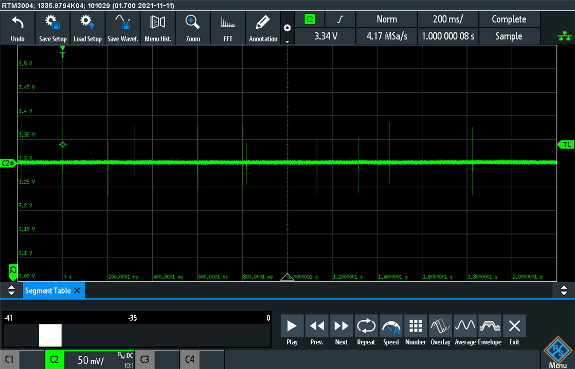
This then had me wondering what the I2C line looked like. The MKR couldn’t do 1MHz, but the Pi could – was it borderline? Not having the PEC enabled means that errors would slip through silently, but reduces processing load. I had previously verified that a change in speed didn’t change the dip behaviour, but since I had the oscilloscope out, it would be nice to take a look.
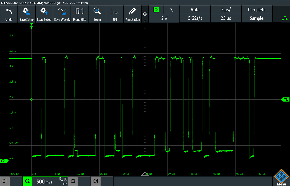
While not the cleanest and looking at just SDA, the result is still clearly a binary signal and the acknowledges from both ends are coming through – the Click board pulling down to about 350mV while the PI pulls down to 150mV suggesting the Pi has the better drive strength. Bus errors seemed relatively unlikely at this point.
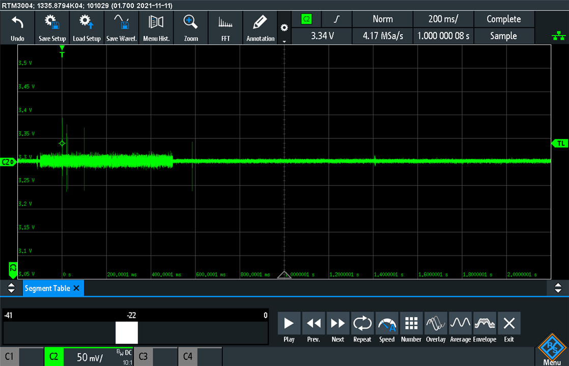
This was when I realised that in probing the I2C line for signal quality, somehow the Raspberry Pi’s readings were no longer spiky. Probing the board fixed the problem? Aha!
Eureka! Alien Signal Identified!
If you’ve been following along, you may well have identified the alien signal already by the time I finished the first experiment. Indeed, I had an inkling already as of the first experiment, but I proceeded to try eliminating all other causes.
The cause of the signal was an unexpected one. As I run my Raspberry Pi from a good quality USB wall charger, it has an isolated, floating output. Similarly, the outputs from my test equipment are also isolated, floating outputs. That would seem fine, right?
In fact, it seems that it wasn’t fine. Instead, my hypothesis is that everything floating may mean that charge could have accumulated from external sources such as the environment around the circuit and created common-mode voltage offsets enough that it would have found a route to equalise. This could be through a chip or via some capacitive path (as is often found in power supplies). The fact I saw a signal at 3-4Hz may indicate that the charge was building up at a nearly constant rate to a threshold and then “dumping” through something to equalise. That might have created enough of a disturbance to the chip thus causing the “spike” to appear.
Grounding the circuit would allow a path for these charges to be equalised so that they do not build up and seemed to resolve the issue. Initially, this ground path was (unintentionally) provided through a USB cable to a desktop computer where the DC ground is common with the mains ground. Further testing also “accidentally” provided a ground when testing the I2C bus with an oscilloscope, whereby it was observed that readings were good. For further tests, an intentional low-impedance ground was provided using a thick gauge wire and alligator clip from the SMU’s mains ground connector to the Pi 3 Click Shield ground test loop.
The New (Correct) Results
The experiment was repeated, following the same methodology as in the prior blog posting, using a Keithley 2450 SourceMeter and a Rohde & Schwarz NGM202 Power Supply. The Click was used on the Raspberry Pi 3 B platform to be consistent with the previous (as it still achieves the best throughput). As a reminder, based on the datasheet and information I have to hand, I am expecting the current sensing accuracy to be around 1% to 2%, and voltage sensing accuracy to be about 0.2% to 1.2%.
Current Measurement Accuracy – 1A Range
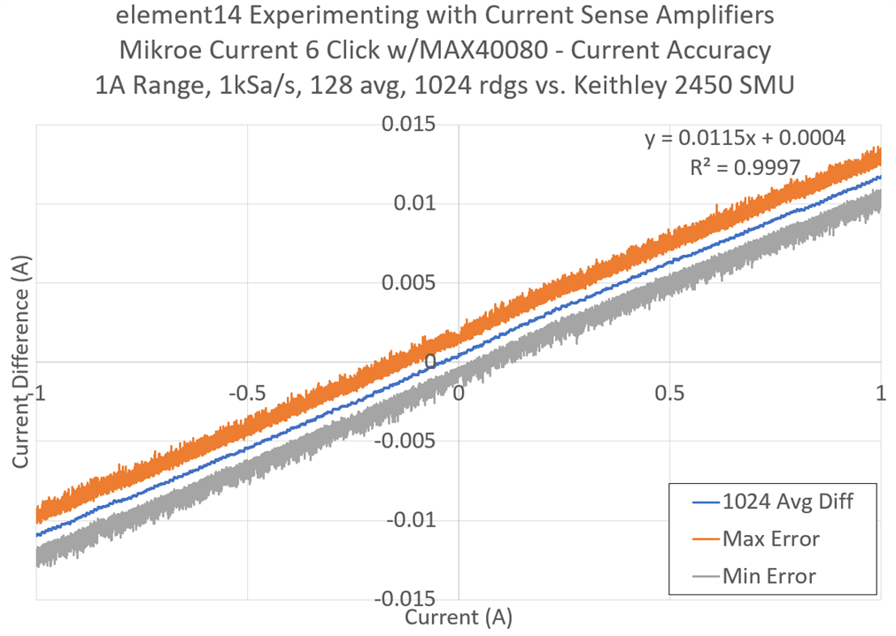
In the 1A range, the result is very linear, achieving an R2 of 0.9997. The gain error is calculated to be 1.15%, of which the bulk may be due to the resistor which is a 1% tolerance part. The offset is quite small at just 0.4mA, considering the 12-bit + sign resolution creates steps of 0.24mA. The single (128-average) reading error can deviate from the average about ±1.5mA which is more noticeable and suggests that this may not be ideal for applications profiling small currents or where single (128-average) readings must be more accurate.
Current Measurement Accuracy – 5A Range
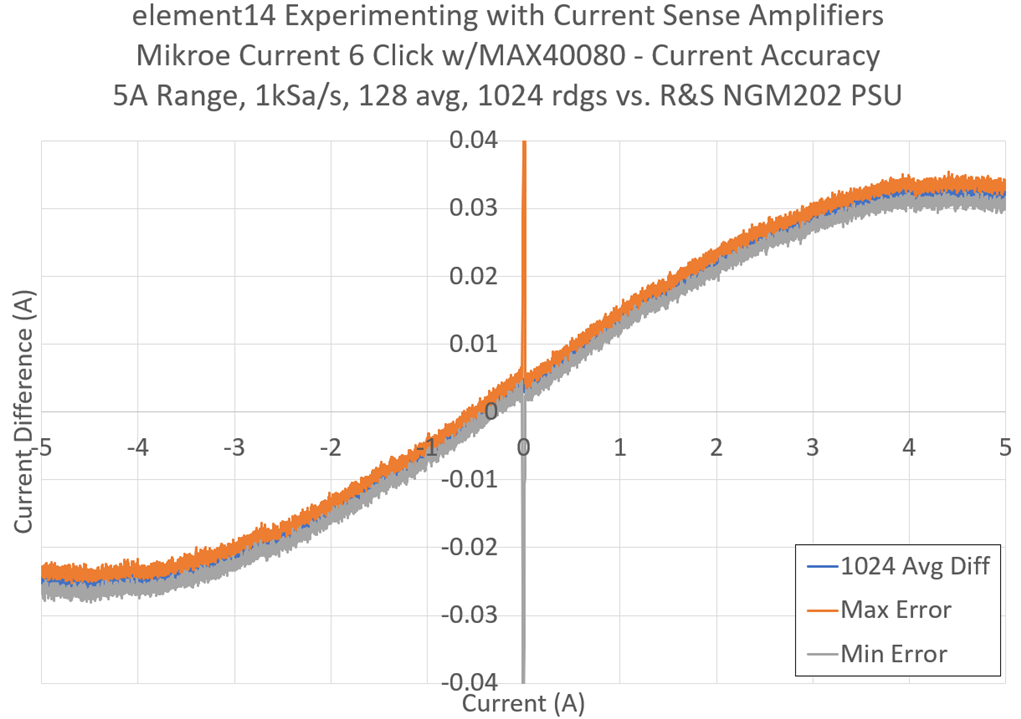
Repeating the same for the 5A range, the curve deviates significantly when higher currents are used. This suggests this error is likely to be induced through the effect of shunt heating due to the choice of resistor and design of the Current 6 Click and is not intrinsic to the MAX40080. An error spike is seen around zero – this is likely due to the NGM202’s accuracy around zero and the fact that the positive and negative current is measured in two separate runs with manual reversal of the leads, as the NGM202 is a two-quadrant supply.
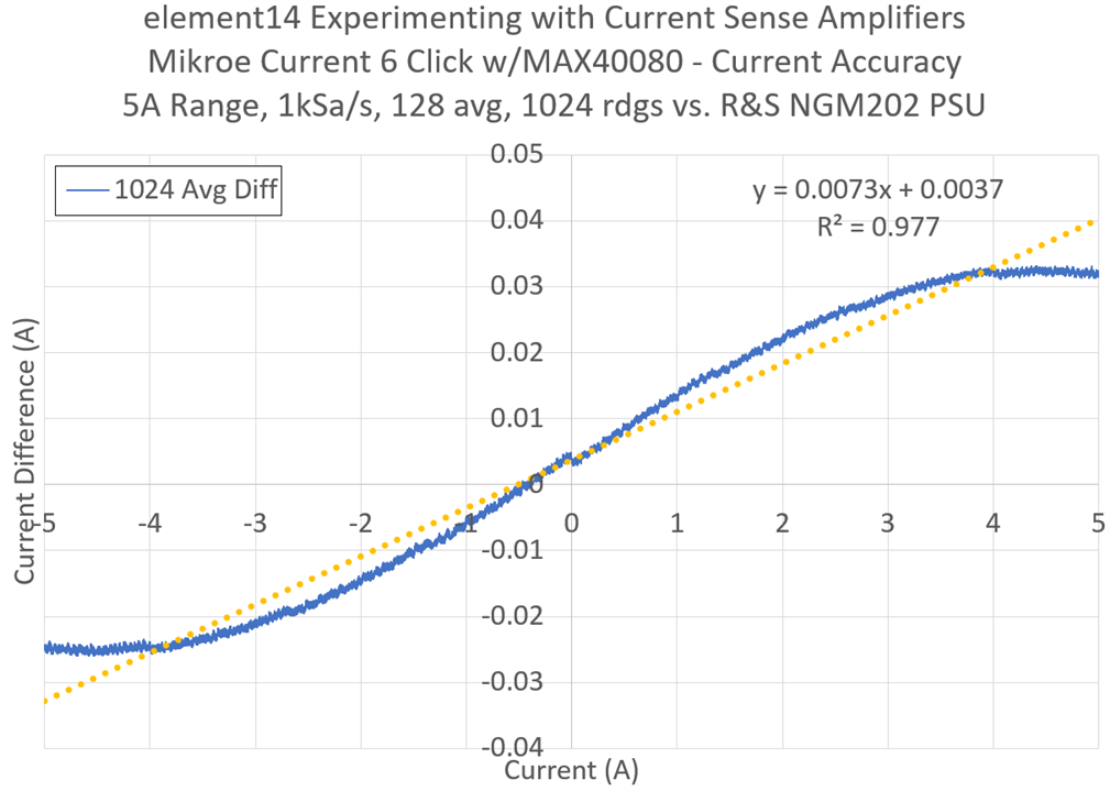
The linear fit is now less linear, with an R2 of 0.977. The gain error is quite impressive at 0.73% with a 3.7mA offset. The gain error is excellent and the offset is within range.
Voltage Measurement Accuracy
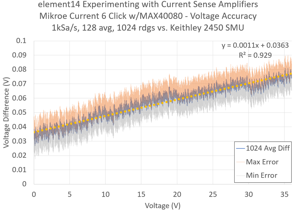
Repeating the voltage accuracy tests shows a similar result within the boundary of error. The voltage gain error is 0.11% with a 36.3mV offset, the latter of which is just slightly above the datasheet maximum. The cause may well have been the SMU which has a 10mV offset specification in addition to thermal EMFs. The result is excellent and is likely to be within specification.
Current Measurement Noise – 1A Range
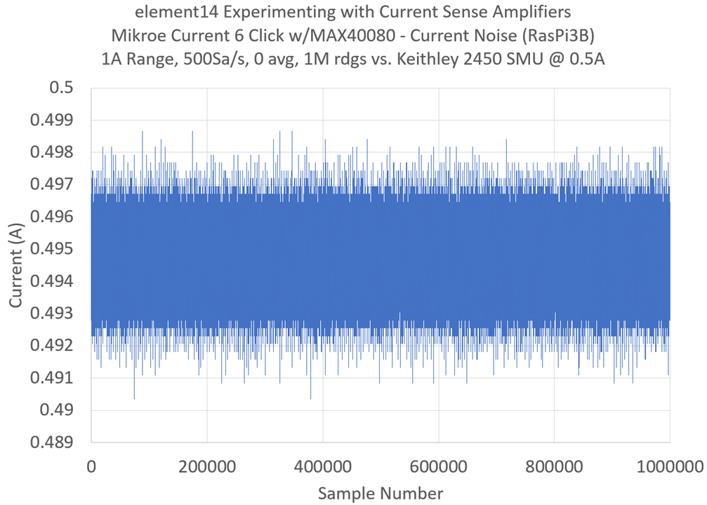
Current noise in the 1A range is now very tame and looks like classic ADC noise. With 0.5A input in the 1A range, the peak-to-peak value measured 8.3mA with an RMS value of 0.75mA. There were no temporal patterns identified in the data.

The histogram shows a bell-like distribution which is exactly what is expected when operating correctly.
Current Measurement Noise – 5A Range
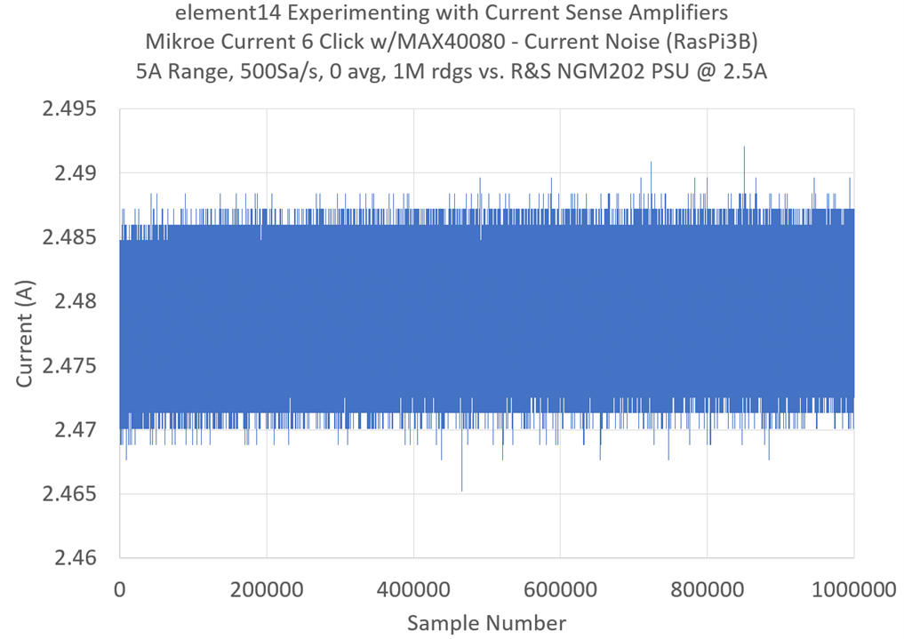
In the 5A range, a slight “rise” in the value is seen at the beginning due to shunt heating. The peak-to-peak noise is 26.9mA with an RMS of 3.1mA. No temporal patterns were seen.

The histogram is not quite a bell-curve distribution, likely due to the “shift” in actual measurement caused by shunt heating. It is still relatively “tight” overall.
Voltage Measurement Noise
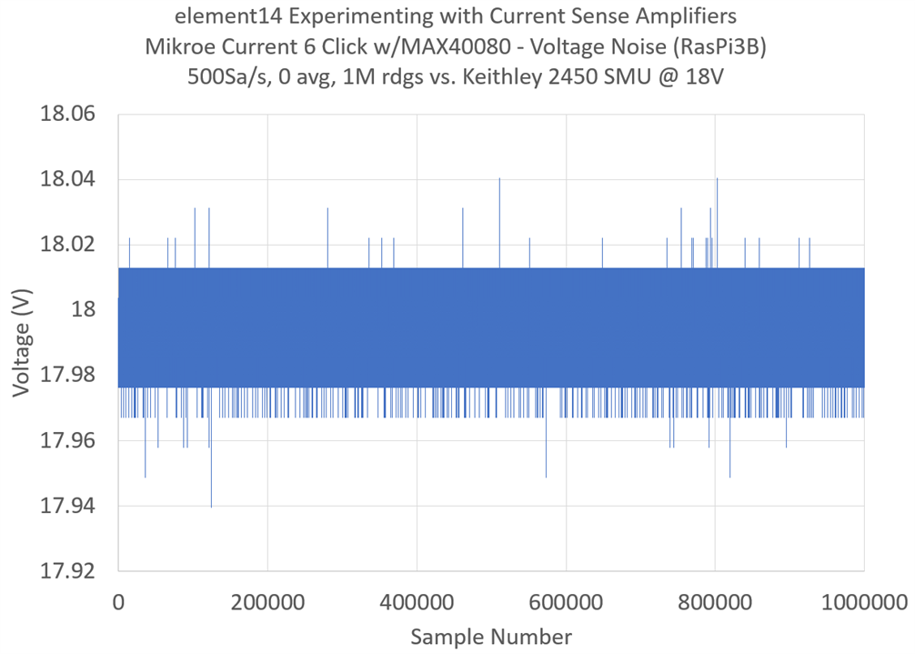
The voltage measurement noise is relatively small, thus the quantisation of the ADC becomes visible in the data. Of note is that due to the gain factor, full-scale ADC corresponds to 37.5V while the allowable range is up to 36V, resulting in a quantisation of 9.16mV per step. The measured peak-to-peak noise was 100.7mV, mostly due to singular spikes, with an RMS value of just 8.05mV. The performance is excellent overall to the point that a histogram really is not needed.
Conclusion
It seems I was mistaken in the end and I feel like I owe the MAX40080 and Current Click 6 a bit of an apology for the poor showing in the previous blog posting. It turns out it was a case of mea culpa because of the hardware configuration even though it was not obvious to me at first. In short, ground the Raspberry Pi to avoid potential noise (which I presume could arise due to induced stray charges which might be creating common-mode voltages which eventually find a path to equalise).
Once a proper ground was supplied at one point in the circuit, measured accuracy results were significantly improved.
In the 1A range, a gain error of 1.15% with an offset of 0.4mA was registered. In the 5A range, this was 0.73% and 3.7mA respectively. Voltage measurements had a gain error of 0.11% and 36.3mV offset, much of that likely from the power supply. Noise-wise, at 1A, 8.3mA peak-to-peak and 0.75mA RMS was recorded. At 5A, this was 26.9mA and 3.1mA respectively. Measuring voltage, this was 100.7mV and 8.05mV respectively. The results overall are excellent and within expectations.
However, the issue of achieving high sample rates proved somewhat elusive. Trying to use an Arduino MKR1010 Wi-Fi board with the Click with jumper wiring saw bus rates of up to 900kHz possible, above which data corruption occurred. Disabling PEC and operating based on “hammering” the FIFO only, passing only valid reading bytes over the USB (virtual) CDC serial interface to minimise the work required still did not achieve sample rates surpassing that of the Raspberry Pi + Python solution. This was due to the processing time required for the SoC to perform a USB transaction which reduced the sample rate from about 17.7kHz down to 9.7kHz in practice. If the Arduino is required to translate readings into an ASCII value, a sample rate closer to 4.5kHz (on average) is achieved. The Raspberry Pi-based platform still performs better, with fewer optimisations, in part due to the higher compute power available even though it is running a full multi-tasking operating system.
The adventure continues – in a future blog posting, I will likely apply the current-sensing amplifier to profiling higher-consumption consumer electronics. If time permits, I’ll see if things get better changing over to a C-based program on the Raspberry Pi to remove the Python overhead, but I suspect the gains may still be limited.
Incidentally, this is a good demonstration of what can happen when I start reviewing things "progressively" - I can end up with results that don't make sense and end up publishing them anyway, only to have to re-do them later. This is a prime example of why I prefer delivering my RoadTests as a monolithic "lump" near the due date, rather than trying to write blogs as I go along. Perhaps some of you enjoy this adventure ... but for me, I feel this misstep was a regrettable mistake ...
---
This is part of the Experimenting with Current Sense Amplifiers Design Challenge – A Current-Sensing PSU Upgrade Blog Series:
- Blog #1: A Current-Sensing PSU Upgrade - Introduction
- Blog #2: A Current-Sensing PSU Upgrade - Unboxing
- Blog #3: A Current-Sensing PSU Upgrade – Setting Up
- Blog #4: A Current-Sensing PSU Upgrade – Accuracy & Noise Performance
- Blog #5: A Current-Sensing PSU Upgrade – Arduino Gets Involved, Ground to Raspberry Pi … Alien Signal Identified!
- Blog #6: A Current-Sensing PSU Upgrade – PSU Logging, CSA & FastLog Comparison, a Sound Check & an Overall Summary
