


Can IIR FIlters Be Fully Pipelined?
We have reached the final post in this series on LWDF IIR filters. I hope that I was able to convince you that many, if not all, of the perceived disadvantages of IIR filters can be addressed while maintaining their one major advantage over their more popular FIR cousins, i.e. much lower filter size needed to meet given specifications.
As a quick recap, especially in their LWDF polyphase form, these IIR filters are very efficient, unconditionally stable, have good coefficient quantization sensitivity properties, and there are many clever ways to achieve almost linear phase, IIR's number one drawback when compared to FIRs.
One weak point remaining is achieving very high sample rates, ideally equal to the clock rate at the data sheet fMAX spec. While efficient ways of pipelining all-pass first and second order sections that maximize throughput do exist, namely replacing every delay in the design with four delays (or two in the bireciprocal case), this does not increase the sample rate, which remains a quarter respectively half the clock rate, instead increases the number of channels from one to four respectively two. Yes, this is a very good way to use the available DSP resources efficiently but sample rates equal to the clock rate remain an impossible goal. The main impediment is the tight feedback loop inherent to all IIR filters, with one (or two in the bireciprocal case) delays in that loop, which seems like an insurmountable barrier.
The good news is that if sample rate equal to the clock frequency is the main goal and if it must be achieved at all costs, any IIR can be pipelined to reach that high sample rate. You might not like the price that needs to be paid for that, but a solution does exist.
I will show now how this can be done for the three all-pass filter building blocks, the first order, second order and second order bireciprocal. The goal is to modify the design so that we have four delays in the feedback loop, with a single channel implementation. Let's start with the easiest case, the second order bireciprocal all-pass section:
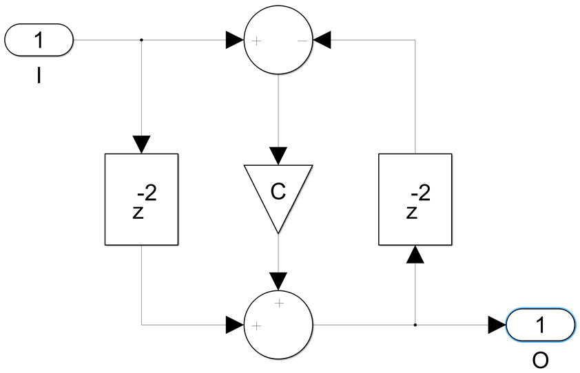
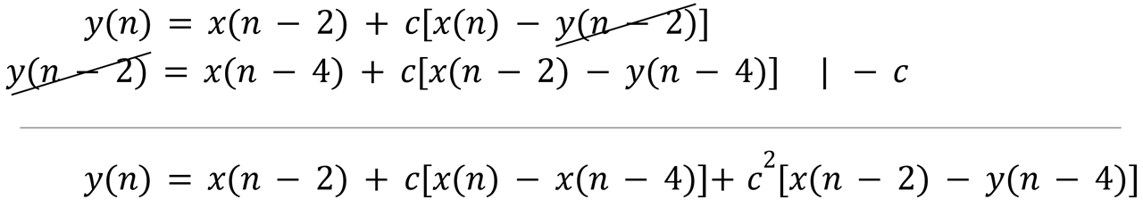
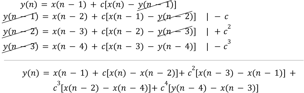
We can see that there are only two delays in the feedback loop, and we need four. We start with the finite difference equation corresponding to this architecture:
![]()
The problem here is that y(n) is a function of y(n-2) and we would like to have y(n-4) instead. This can be done if we substitute y(n-2) as a function of y(n-4) in this equation. We write the two equations together, we multiply the second one by -c, add them and y(n-2) cancels out:
This now meets the goal of having four delays in the feedback loop but the price is twice as many additions and multiplications. It fits neatly into two DSP primitives and to be clear, this is a single channel, running now at a sample rate equal to the clock frequency:
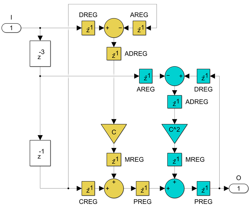
Since the first order bireciprocal all-pass section is simply a delay, this solves the maximum sample rate being half the clock frequency problem for all LWDF bireciprocal filters. We have doubled the sample rate at the price of doubling the number of DSP primitives being used.
The next case to consider is the first order non-bireciprocal all-pass section:
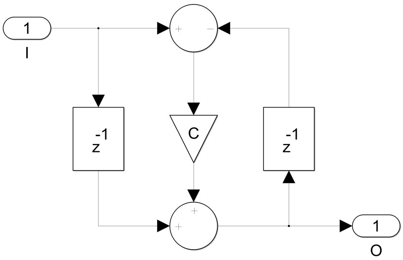
Here we have only one delay in the feedback loop and we want four. If we were to pipeline this with the usual technique of replacing each delay with four delays, we can run at full clock speed but we get four channels, each one running at a sample rate equal to a quarter of the clock frequency. We apply the same math trick to the finite difference equation, but four times, the goal is to remove the dependency of y(n) on y(n-1), y(n-2) and y(n-3) so that only y(n-4) remains:
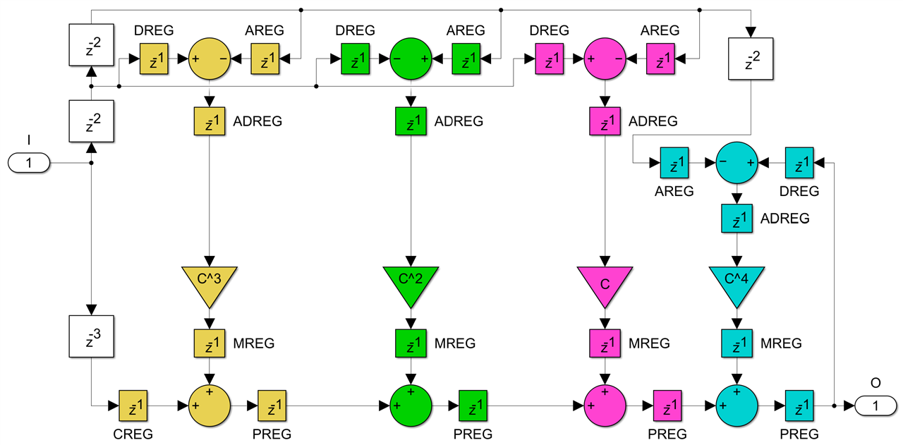
We achieve the goal for a single channel running at the full clock speed instead of four channels running at a quarter of the clock frequency, but we need to use four DSPs instead of just one:
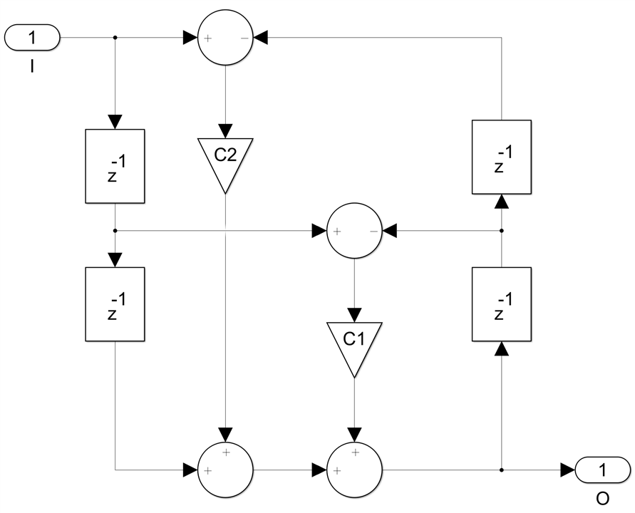
Finally, the most complicated case is the second order non-bireciprocal all-pass section, the one with two coefficients:
I will not bore you with the gory high school algebra details, but the main idea is the same, you start with the finite difference equation:

and combine it with delayed versions of it, cancelling all y(n-1), y(n-2) and y(n-3) terms, which yields the scary looking formula:
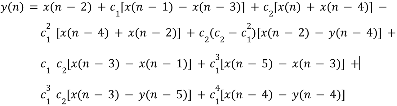
There are nine terms now, all but one corresponding to one DSP, with the portions in square brackets mapping to pre-adders. The eight DSPs are connected in one long post-adder chain, with x(n-2) driving the C port of the first DSP. The eight coefficients can of course be pre-computed, so that costs nothing. I will leave the actual pipelined DSP structure for this case as an exercise for the interested reader.
Like in the first order all-pass section case, a sample rate equal to the clock rate is now possible, the cost being 4 times more DSP resources, 8 instead of just 2. You only need these versions if sample speeds in the 250Msps to 1Gsps range are required, otherwise the four-channel fully pipelined versions described in Post 23 are enough and four times more efficient in terms of DSP utilization.
In conclusion, while FIR filters definitely have their place, people ignore more efficient IIR filter implementations at their own cost. In particular, if you find yourself designing and using FIRs of order N=64 or higher, you shouldn't - there are usually better ways to achieve the same result.
Back to the top: The Art of FPGA Design Season 2
