BeeWatch: LoRaWAN Environmental Monitoring – Blog 10: Nicla Vision Power, Saving B’s & Dashboard Woes

As we count down the days to the end of the Save the Bees Design Challenge, a regret I carry from my last post is that I didn’t attempt any AI-based inferencing now that I have a Nicla Vision board in my hand. In this post, we’ll try to change this while also trying to tie up the last few stretch goals in my proposal.

Nicla Vision Power Requirements

A lot of people are enthusiastic about AI’s use, but we all know that such models can be quite computationally intensive. As a result, I was curious about the Nicla Vision’s power requirements while running some of the example code and code of my own. To measure this, as it requires a USB data connection to use interactively, I used a USB power meter (specifically, the highly-accurate FNB58 which was recommended by scottiebabe  which I am still reviewing at this time).

My results are as follows:

It would seem that based on these results, while the board is busy with MJPEG streaming and Wi-Fi, it can consume the better part of 1W. When it is in deep sleep, it’s still consuming close to 0.1W in spite of being (logically) disconnected from USB as the host processor is stopped. Granted the power consumption when powered from the battery header may be lower due to the design reducing quiescent draw, but I think it does show that AI and computer vision does not come cheap with regards to power. It is interesting to see the MQTT code consumes more power than the Edge Impulse code – this may be because it’s using Wi-Fi while the Edge Impulse code is not using Wi-Fi. If both are in use, I’d expect power requirements to increase beyond this.

Assuming it’s running some inferencing at 0.7W for 24/7, this will consume 16.8Wh of energy, which would translate to 4541mAh from a 3.7V Li-Ion cell assuming perfect 100% energy conversion. In the case of solar energy, assuming a place with about 4-peak-sun-hours on average (as per my latitude), it would require 4.2W of panel just to meet the requirements. In reality, a bit more is required and around five-times the daily usage in battery storage is required to ensure a very high (99.999%) availability when given the statistical run of adverse weather and cloudy days (so a 25,000mAh “brick” of cells like a power bank would be needed). It’s not impossible, but it makes the LoRaWAN board look like a feather by comparison when it comes to power.

Saving the “B’s”

I decided it was time to stop resisting and just start getting my toes wet with AI through Edge Impulse. But at first, one has to be able to walk, before they can run. That is why I decided to devise a simple classification project that would be easy to get a lot of data for and hopefully work.

That is where I had a brain-wave. What if instead of saving bees, I would just save B’s. At least, that way, I could tell other people I was saving bees and they’d be none the wiser! Best of all, B’s are easy to come by while bees are not! After all, you can’t save bees without the letter B!

As a result, I started off by downloading ImageMagick, a command-line image manipulation tool I would be using to generate my B’s and notB’s. The first step was to get it to list all the fonts on my system using the convert -list font command. Then, I piped that into a trivial Python program to build a Python “list” of fonts in a second program. This second program is responsible for getting a list of labels and creating PNG files containing the letter in question – the below example generates the set of notB’s for my particular system:

import subprocess
import shlex

fontlist = ["Agency-FB",
"Agency-FB-Bold",
"Algerian",
"Arial",
"Arial-Black",
"Arial-Bold",
"Arial-Bold-Italic",
"Arial-Italic",
"Arial-Narrow",
"Arial-Narrow-Bold",
"Arial-Narrow-Bold-Italic",
"Arial-Narrow-Italic",
"Arial-Rounded-MT-Bold",
"Bahnschrift",
"Baskerville-Old-Face",
"Bauhaus-93",
"Bell-MT",
"Bell-MT-Bold",
"Bell-MT-Italic",
"Berlin-Sans-FB",
"Berlin-Sans-FB-Bold",
"Berlin-Sans-FB-Demi-Bold",
"Bernard-MT-Condensed",
"Blackadder-ITC",
"Bodoni-MT",
"Bodoni-MT-Black",
"Bodoni-MT-Black-Italic",
"Bodoni-MT-Bold",
"Bodoni-MT-Bold-Italic",
"Bodoni-MT-Condensed",
"Bodoni-MT-Condensed-Bold",
"Bodoni-MT-Condensed-Bold-Italic",
"Bodoni-MT-Condensed-Italic",
"Bodoni-MT-Italic",
"Bodoni-MT-Poster-Compressed",
"Book-Antiqua",
"Book-Antiqua-Bold",
"Book-Antiqua-Bold-Italic",
"Book-Antiqua-Italic",
"Bookman-Old-Style",
"Bookman-Old-Style-Bold",
"Bookman-Old-Style-Bold-Italic",
"Bookman-Old-Style-Italic",
"Bookshelf-Symbol-7",
"Bradley-Hand-ITC",
"Britannic-Bold",
"Broadway",
"Brush-Script-MT-Italic",
"Calibri",
"Calibri-Bold",
"Calibri-Bold-Italic",
"Calibri-Italic",
"Calibri-Light",
"Calibri-Light-Italic",
"Californian-FB",
"Californian-FB-Bold",
"Californian-FB-Italic",
"Calisto-MT",
"Calisto-MT-Bold",
"Calisto-MT-Bold-Italic",
"Calisto-MT-Italic",
"Cambria-&-Cambria-Math",
"Cambria-Bold",
"Cambria-Bold-Italic",
"Cambria-Italic",
"Candara",
"Candara-Bold",
"Candara-Bold-Italic",
"Candara-Italic",
"Candara-Light",
"Candara-Light-Italic",
"Castellar",
"Centaur",
"Century",
"Century-Gothic",
"Century-Gothic-Bold",
"Century-Gothic-Bold-Italic",
"Century-Gothic-Italic",
"Century-Schoolbook",
"Century-Schoolbook-Bold",
"Century-Schoolbook-Bold-Italic",
"Century-Schoolbook-Italic",
"Chiller",
"Colonna-MT",
"Comic-Sans-MS",
"Comic-Sans-MS-Bold",
"Comic-Sans-MS-Bold-Italic",
"Comic-Sans-MS-Italic",
"Consolas",
"Consolas-Bold",
"Consolas-Bold-Italic",
"Consolas-Italic",
"Constantia",
"Constantia-Bold",
"Constantia-Bold-Italic",
"Constantia-Italic",
"Cooper-Black",
"Copperplate-Gothic-Bold",
"Copperplate-Gothic-Light",
"Corbel",
"Corbel-Bold",
"Corbel-Bold-Italic",
"Corbel-Italic",
"Corbel-Light",
"Corbel-Light-Italic",
"Courier-New",
"Courier-New-Bold",
"Courier-New-Bold-Italic",
"Courier-New-Italic",
"Curlz-MT",
"Dubai-Bold",
"Dubai-Light",
"Dubai-Medium",
"Dubai-Regular",
"Ebrima",
"Ebrima-Bold",
"Edwardian-Script-ITC",
"Elephant",
"Elephant-Italic",
"Engravers-MT",
"Eras-Bold-ITC",
"Eras-Demi-ITC",
"Eras-Light-ITC",
"Eras-Medium-ITC",
"Felix-Titling",
"Footlight-MT-Light",
"Forte",
"Franklin-Gothic-Book",
"Franklin-Gothic-Book-Italic",
"Franklin-Gothic-Demi",
"Franklin-Gothic-Demi-Cond",
"Franklin-Gothic-Demi-Italic",
"Franklin-Gothic-Heavy",
"Franklin-Gothic-Heavy-Italic",
"Franklin-Gothic-Medium",
"Franklin-Gothic-Medium-Cond",
"Franklin-Gothic-Medium-Italic",
"Freestyle-Script",
"French-Script-MT",
"Gabriola",
"Gadugi",
"Gadugi-Bold",
"Garamond",
"Garamond-Bold",
"Garamond-Italic",
"Georgia",
"Georgia-Bold",
"Georgia-Bold-Italic",
"Georgia-Italic",
"Gigi",
"Gill-Sans-MT",
"Gill-Sans-MT-Bold",
"Gill-Sans-MT-Bold-Italic",
"Gill-Sans-MT-Condensed",
"Gill-Sans-MT-Ext-Condensed-Bold",
"Gill-Sans-MT-Italic",
"Gill-Sans-Ultra-Bold",
"Gill-Sans-Ultra-Bold-Condensed",
"Gloucester-MT-Extra-Condensed",
"Goudy-Old-Style",
"Goudy-Old-Style-Bold",
"Goudy-Old-Style-Italic",
"Goudy-Stout",
"Haettenschweiler",
"Harlow-Solid-Italic",
"Harrington",
"High-Tower-Text",
"High-Tower-Text-Italic",
"Holo-MDL2-Assets",
"Impact",
"Imprint-MT-Shadow",
"Informal-Roman",
"Ink-Free",
"Javanese-Text",
"Jokerman",
"Juice-ITC",
"Kristen-ITC",
"Kunstler-Script",
"Leelawadee-UI",
"Leelawadee-UI-Bold",
"Leelawadee-UI-Semilight",
"Lucida-Bright",
"Lucida-Bright-Demibold",
"Lucida-Bright-Demibold-Italic",
"Lucida-Bright-Italic",
"Lucida-Calligraphy-Italic",
"Lucida-Console",
"Lucida-Fax-Demibold",
"Lucida-Fax-Demibold-Italic",
"Lucida-Fax-Italic",
"Lucida-Fax-Regular",
"Lucida-Handwriting-Italic",
"Lucida-Sans-Demibold-Italic",
"Lucida-Sans-Demibold-Roman",
"Lucida-Sans-Italic",
"Lucida-Sans-Regular",
"Lucida-Sans-Typewriter-Bold",
"Lucida-Sans-Typewriter-Bold-Oblique",
"Lucida-Sans-Typewriter-Oblique",
"Lucida-Sans-Typewriter-Regular",
"Lucida-Sans-Unicode",
"Magneto-Bold",
"Maiandra-GD",
"Malgun-Gothic",
"Malgun-Gothic-Bold",
"Malgun-Gothic-SemiLight",
"Matura-MT-Script-Capitals",
"Microsoft-Himalaya",
"Microsoft-JhengHei-&-Microsoft-JhengHei-UI",
"Microsoft-JhengHei-Bold-&-Microsoft-JhengHei-UI-Bold",
"Microsoft-JhengHei-Light-&-Microsoft-JhengHei-UI-Light",
"Microsoft-New-Tai-Lue",
"Microsoft-New-Tai-Lue-Bold",
"Microsoft-PhagsPa",
"Microsoft-PhagsPa-Bold",
"Microsoft-Sans-Serif",
"Microsoft-Tai-Le",
"Microsoft-Tai-Le-Bold",
"Microsoft-YaHei-&-Microsoft-YaHei-UI",
"Microsoft-YaHei-Bold-&-Microsoft-YaHei-UI-Bold",
"Microsoft-YaHei-Light-&-Microsoft-YaHei-UI-Light",
"Microsoft-Yi-Baiti",
"MingLiU-ExtB-&-PMingLiU-ExtB-&-MingLiU_HKSCS-ExtB",
"Mistral",
"Modern-No.-20",
"Mongolian-Baiti",
"Monotype-Corsiva",
"MS-Gothic-&-MS-UI-Gothic-&-MS-PGothic",
"MS-Outlook",
"MS-Reference-Sans-Serif",
"MS-Reference-Specialty",
"MT-Extra",
"MV-Boli",
"Myanmar-Text",
"Myanmar-Text-Bold",
"Niagara-Engraved",
"Niagara-Solid",
"Nirmala-UI",
"Nirmala-UI-Bold",
"Nirmala-UI-Semilight",
"OCR-A-Extended",
"Old-English-Text-MT",
"Onyx",
"Palace-Script-MT",
"Palatino-Linotype",
"Palatino-Linotype-Bold",
"Palatino-Linotype-Bold-Italic",
"Palatino-Linotype-Italic",
"Papyrus",
"Parchment",
"Perpetua",
"Perpetua-Bold",
"Perpetua-Bold-Italic",
"Perpetua-Italic",
"Perpetua-Titling-MT-Bold",
"Perpetua-Titling-MT-Light",
"Playbill",
"Poor-Richard",
"Pristina",
"Rage-Italic",
"Ravie",
"Rockwell",
"Rockwell-Bold",
"Rockwell-Bold-Italic",
"Rockwell-Condensed",
"Rockwell-Condensed-Bold",
"Rockwell-Extra-Bold",
"Rockwell-Italic",
"Sans-Serif-Collection",
"Script-MT-Bold",
"Segoe-Fluent-Icons",
"Segoe-MDL2-Assets",
"Segoe-Print",
"Segoe-Print-Bold",
"Segoe-Script",
"Segoe-Script-Bold",
"Segoe-UI",
"Segoe-UI-Black",
"Segoe-UI-Black-Italic",
"Segoe-UI-Bold",
"Segoe-UI-Bold-Italic",
"Segoe-UI-Emoji",
"Segoe-UI-Historic",
"Segoe-UI-Italic",
"Segoe-UI-Light",
"Segoe-UI-Light-Italic",
"Segoe-UI-Semibold",
"Segoe-UI-Semibold-Italic",
"Segoe-UI-Semilight",
"Segoe-UI-Semilight-Italic",
"Segoe-UI-Symbol",
"Segoe-UI-Variable",
"Showcard-Gothic",
"SimSun-&-NSimSun",
"SimSun-ExtB",
"Sitka-Text",
"Sitka-Text-Italic",
"Snap-ITC",
"Source-Code-Pro",
"Source-Code-Pro-Black",
"Source-Code-Pro-Bold",
"Source-Code-Pro-ExtraLight",
"Source-Code-Pro-Light",
"Source-Code-Pro-Semibold",
"Stencil",
"Sylfaen",
"Symbol",
"Tahoma",
"Tahoma-Bold",
"Tempus-Sans-ITC",
"Times-New-Roman",
"Times-New-Roman-Bold",
"Times-New-Roman-Bold-Italic",
"Times-New-Roman-Italic",
"Trebuchet-MS",
"Trebuchet-MS-Bold",
"Trebuchet-MS-Bold-Italic",
"Trebuchet-MS-Italic",
"Tw-Cen-MT",
"Tw-Cen-MT-Bold",
"Tw-Cen-MT-Bold-Italic",
"Tw-Cen-MT-Condensed",
"Tw-Cen-MT-Condensed-Bold",
"Tw-Cen-MT-Condensed-Extra-Bold",
"Tw-Cen-MT-Italic",
"Verdana",
"Verdana-Bold",
"Verdana-Bold-Italic",
"Verdana-Italic",
"Viner-Hand-ITC",
"Vivaldi-Italic",
"Vladimir-Script",
"Webdings",
"Wide-Latin",
"Wingdings",
"Wingdings-2",
"Wingdings-3",
"Yu-Gothic-Bold-&-Yu-Gothic-UI-Semibold-&-Yu-Gothic-UI-Bold",
"Yu-Gothic-Light-&-Yu-Gothic-UI-Light",
"Yu-Gothic-Medium-&-Yu-Gothic-UI-Regular",
"Yu-Gothic-Regular-&-Yu-Gothic-UI-Semilight",
"ZWAdobeF"]
labellist = ["a","c","d","e","f","g","h","i","j","k","l","m","n","o","p","q","r","s","t","u","v","w","x","y","z",
"A","C","D","E","F","G","H","I","J","K","L","M","N","O","P","Q","R","S","T","U","V","W","X","Y","Z",
"1","2","3","4","5","6","7","8","9","0"]
command = "convert.exe"
n = 0

for labelchoice in labellist:
  for fontchoice in fontlist :
    subprocess.call(shlex.split(command+" -background white -fill black -pointsize 24 -font \""+fontchoice+"\" label:"+labelchoice+" \""+labelchoice+str(n)+"_"+fontchoice+".png\""))
  n=n+1

After this, I have a folder full of image files with B’s and notB’s. In the below, this is the folder of B’s, although I had to manually pick out some blank images and symbol images from “wingding” style fonts just so as not to contaminate the pool of B’s.

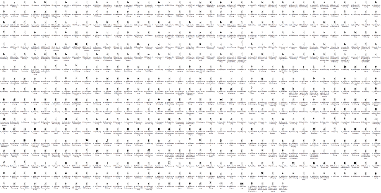
Uploading the full dataset took some time because of its size – in the end 21,159 items were uploaded, most of them being notB’s.

AI Model Training Hyperparameters & Performance

The next step is to build the impulse itself.

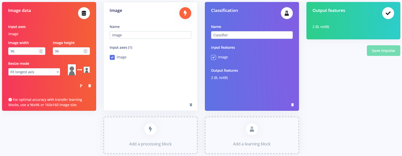
There are a few blocks to choose – the first in the pipeline is an image block. I’ve set it to process such that the images are “fitted” to 96x96 without cropping, so none of the B is lost. However, I did notice that it padded the missing pixels with black, so it may affect the training. The next is the actual model – both classifier and transfer learning seemed to be good fits. The classifier module lets us design our models directly while the transfer learning block appears to let us use pre-trained/configured networks with our data (mostly scaled variants of MobileNetV1/V2).

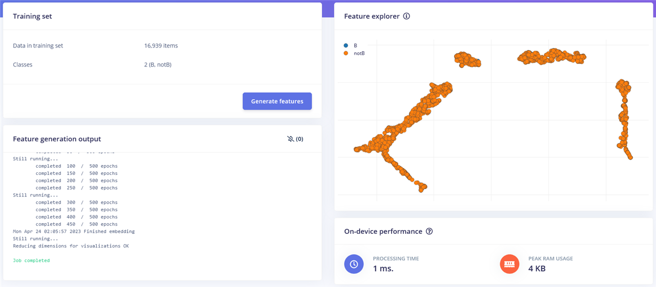
Before we can train, we need to generate features for the model to ingest. The feature map seems to cluster things, but I’m not sure how and both B’s and notB’s are overlapping which is not a great thing (with my naïve understanding of AI).

Transfer Learning

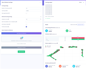
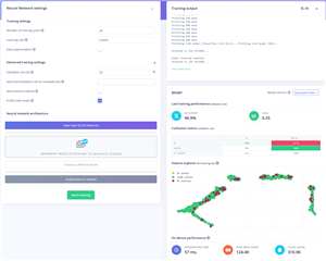
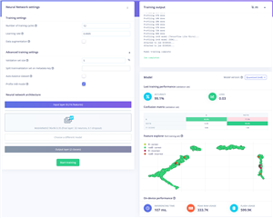
I’ve heard great things about MobileNet and its ability to be both light on resources and having good model performance overall. I decided to give it a go with a range of settings. I tried to maximise the number of epochs within the 20-minute execution time limit. As for the other settings, I did change some of them (learning rate, auto balance, validation set size) but not in any systematic way. It seems what they say about AI optimisation is true – the optimisation of hyperparameters is a time-consuming exercise and can be more of a dark art than a science, as some trends are not trends at all – it may just boil down to a different split between training and testing.

All I can conclude from this is that it seems MobileNetV1 is just terrible at this exercise. While it seems to have high accuracy figures, look at the shocking accuracy for reporting a B when given a B. I’ve seemed to make a thing that says “notB” for everything! Perhaps that’s not wrong – the dataset does have a lot more “notB” than it does “B”, so perhaps the balance dataset option would help.

MobileNetV2 seems to do better – but its capability is really only about 83% accurate at spotting B’s and 99.5% at spotting notB’s based on the profiling done post-training.

Classification Model

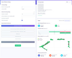
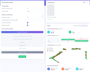
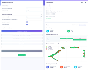
Perhaps we can do better if we just try building our own model types. At this stage, it was like being given a set of levers and pulling at any one in the hopes of making things better. Many times, I made things worse, but eventually I got something which seemed better than the MobileNetV2 result.

In the end, I chose the final tested model here as the one to deploy. We can see that changing validation percentage and keeping other settings the same seems to have resulted in some differences in the profiled accuracy and error figures – purely from changing what the test data is. That’s why small changes in these numbers are not highly meaningful, although it does give me hope that we’re somewhere about 88.5% effective in saving B’s. After all, that’s been about 2.5-hours of CPU training time so far.

Testing & Deploying the Model

The model can be further tested using the Model Testing section in Edge Impulse. This gives us a new perspective into the accuracy figures, as it can run the full testing dataset and indicate which particular examples were inferenced incorrectly and what results are “uncertain”.

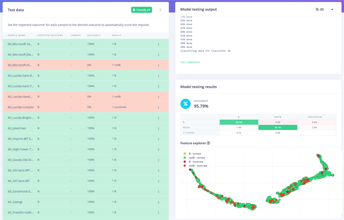
With this, it seems the accuracy is less exciting than I had first thought.

This uncertain example is obviously not a B …

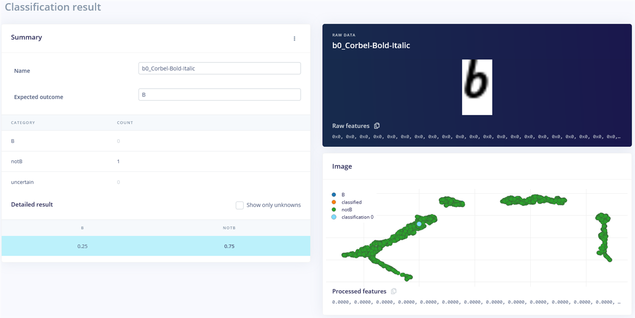
… and this example which is obviously a B is detected as notB. So it seems that AI isn’t quite the “intelligence” we had expected even with figures as high as 97.5% accuracy.

When it came to deploying the model, I was somewhat lost. I had a MobileNetV2 model I wanted to try anyway, but the OpenMV example is for MobileNetV1. I tried downloading the MobileNetV1 tflite model and generated a matching labels file to be copied the OpenMV disk and calling it from the code by modifying the example code but it failed to run with a memory issue.

I was stuck and then I came across this Arduino tutorial for Image Classification with Edge Impulse. It turns out they recommend using the deploy options to generate an OpenMV library which we then have to commit to a forked copy of the OpenMV firmware to build a custom firmware. This seemed a bit painful, but I signed up a GitHub account and forked the repository.

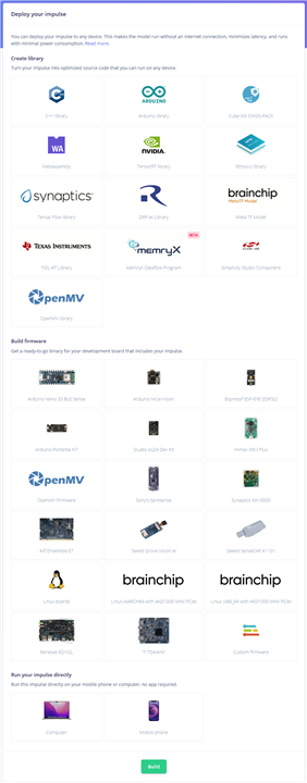
It was only when I was on the deploy screen that I realised that there is an option to deploy to Arduino Nicla Vision directly! Let’s give that a try, but first, let’s deploy to the PC and run it directly in the web browser just to try it with my webcam!

Edit media

Dimensions x Small Medium Large Custom

Subject (required) Brief Description Tags (separated by comma) Video visibility in search results Visible Hidden

Parent content

Design Challenges of The Year - 2023 Wrap Up Winners - Save The Bees Design Challenge BeeWatch: LoRaWAN Environmental Monitoring – Blog 10: Nicla Vision Power, Saving B’s & Dashboard Woes

Poster

Upload Preview

Ok

Cancel

Direct Link: https://www.youtube.com/watch?v=gC2IRGV9PWA

It seems that the object detection type recognition (rather than bounding box) is quite strict on the scale – the letter B is easily misrecognised if it’s not centred or in the exact position it was trained on. Perhaps I should add “noise” into the data by randomly skewing B’s, adding noisy backgrounds, changing the opacity, all in order to make the model a bit more robust. As a result, I don’t have the highest hopes for the model’s real-life use.

Now that the Arduino Nicla Vision export has completed, a ZIP file is received which contains a file to run to program the board with the code. It is noted that you need to install Arduino CLI in order for the script to work.

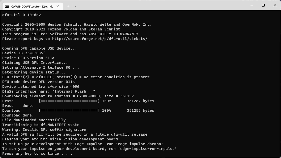
Once loaded onto the board, all one needs is to use a serial monitor and interact with it through AT-commands.

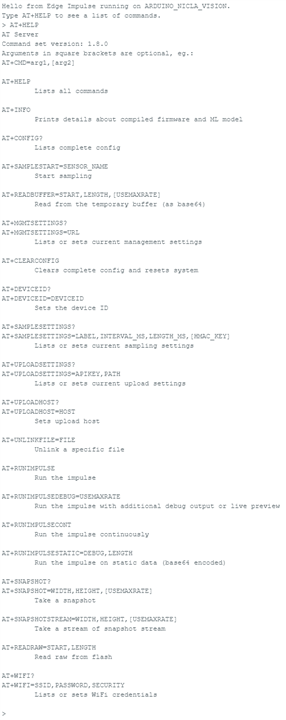
AT+RUNIMPULSE please!

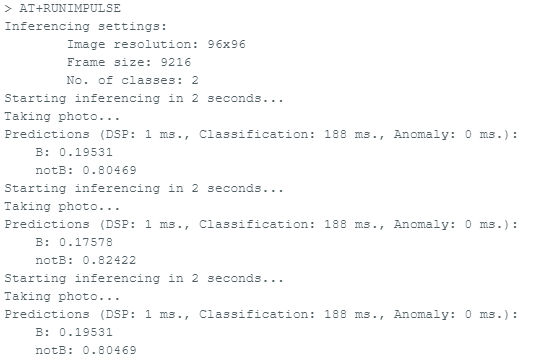
It seems to be working … at least to the point of giving me numbers and not crashing. But it’s hardly easy to use – I can’t see what the camera is seeing in this version, so I think I’ll have to go back to OpenMV.

Thankfully, it seems Edge Impulse can also export to OpenMV just fine and will build a firmware for you without the need for all that GitHub forking and pushing. Once downloading the ZIP file and extracting it, we need to use OpenMV to load the firmware to the board and …

… then it complains the firmware is out of date and offers to upgrade it. Don’t agree to this – otherwise you’ll just wipe the custom firmware that was just loaded! I tried to run the provided .py script and … it fell over.

My interpretation is that there is an issue with the RAM available, so I decided to do a few modifications to the provided .py script to shrink down the image to GRAYSCALE QCIF resolution, then cropped a 96x96 section from it for inferencing as per the model’s desires. Furthermore, I had to enable a rotate and flip so the camera was the right orientation.

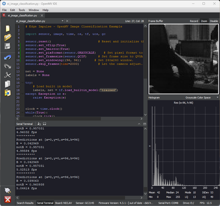
An image at last!

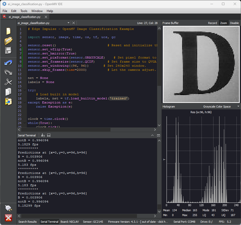
Show it a “D” and it’s clearly 99%+ certain it’s notB.

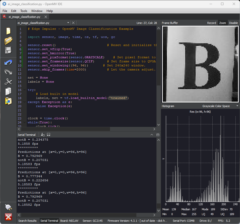
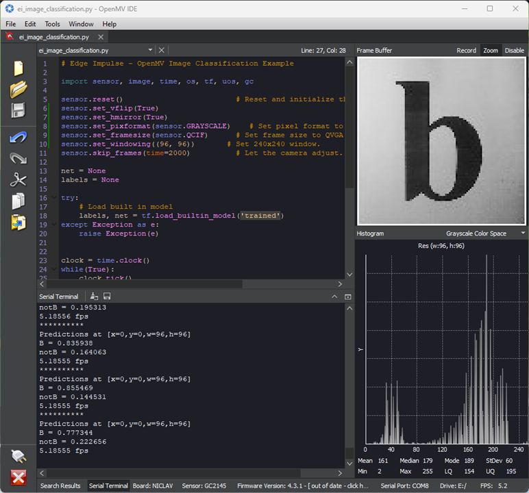
Show it a “B” or a “b” and it seems to be 75-85% certain it’s a B. Given that this is input from a camera rather than a “clean” rendered image, I suppose this is not a horrible outcome.

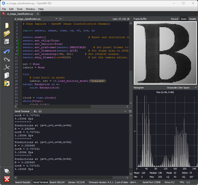
Move a bit too close and now it thinks it’s 70% notB. The brittleness of this model is clear to see!

While in the end, this model probably can’t save any bees as it can’t even robustly detect B’s, at least it’s a first foray into an image classification model running on embedded hardware. Considering I’ve had no exposure to AI development prior to this, it has amazed me that I’ve come so far. However, while Edge Impulse does make things easy to get started, the 20-minute CPU training limit may be part of the reason why certain larger models just cannot be trained on large datasets and be expected to converge when using the free tier. However, the paid options are quite steep – so I think it would be best if steps are documented (or an easy to use distribution is provided) to set-up such a training environment locally instead, as I don’t lack CPU nor GPU resources here.

Attempting a Dashboard

Another stretch goal of mine was to attempt building a dashboard for the data. I’ve previously used NodeRED as part of my RoadTest of a Harting MICA, but I didn’t feel like such a “clunky” solution would be good. Instead, I wanted to investigate other options in case they would be more interesting.

The first was Grafana. I’ve heard great things about its ability to graph and create interactive dashboards. I’ve never used it before, so I signed up for a free account to try it out, hoping it would be straightforward to get it going.

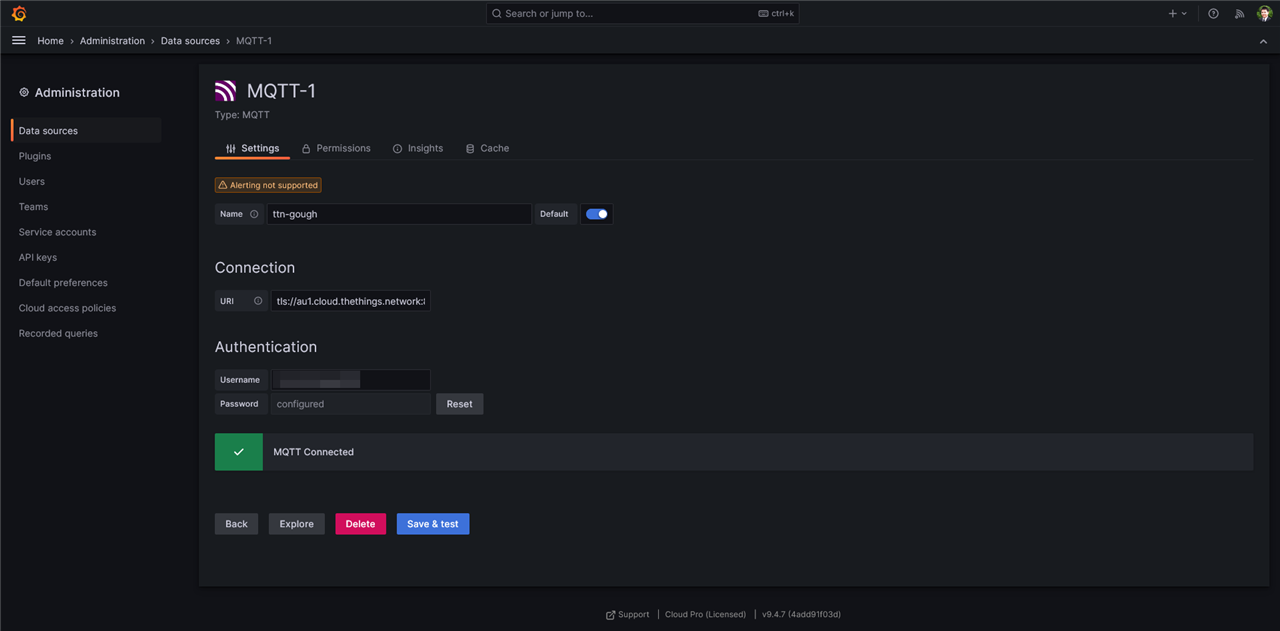
The first thing I tried was simply making an MQTT connection between The Things Network and Grafana, hoping that I could just pull in live data from the topics and get them plotted …

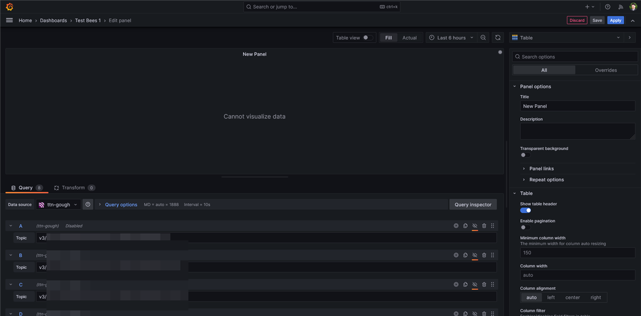
… but alas, I had no luck and I wasn’t sure exactly how to get the data parsed as TTN puts out rather verbose JSON objects that need to be parsed. After some reading, it seems that I also need something in-between (e.g. InfluxDB) to handle the logging of time-series data so that the charts can be zoomed in and out. So much for this being a simple solution …

So I decided to look for something even simpler. How about The MathWorks ThingSpeak? It seems to be a simple data visualisation platform from the company behind MATLAB, and it’s one with built-in integration with The Things Stack –

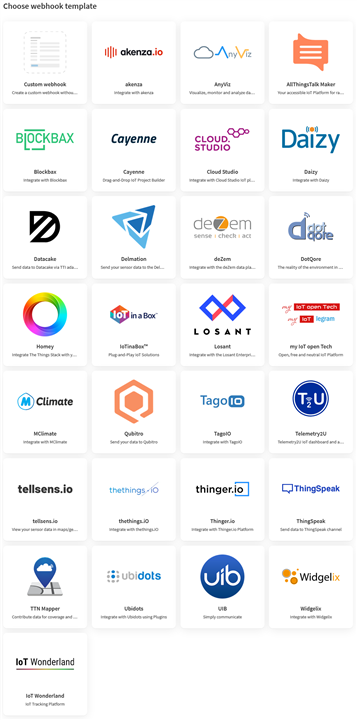
One simply has to sign up for an account, get the API key, create the webhook …

… then modify the JS parsing code to report the data in a particular format. I did all of this, but alas, while ThingSpeak did see the data “push” come through, it couldn’t make sense of any of the data and thus my plots remained empty.

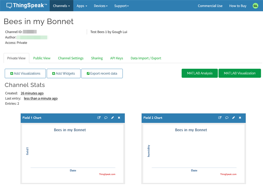
Unfortunately, time is running out and I don’t have the time to fight with this, so I think this stretch-goal was a stretch too far …

The Final Data Dump

As the project draws to a close, to prove the efficacy of my environmental monitors, I’ve decided to consolidate all of the collected environmental data and have it plotted here to show just how long it’s been operating for and the conditions under which it has been running. Two gaps in the data were caused by a loss of MQTT connectivity that was not automatically recovered.

Testing indoors and outdoors show a marked difference in temperature and humidity range. While we are getting into winter, temperatures have been rather stable overall with some range because of weather.

Daily solar variations can be seen depending on the weather, while signal strengths are stable with just one dip which is likely due to interference.

On the whole, the particulate matter level varies quite a bit during the day and is a bit noisy. There are certain days, especially on 22^nd and 23^rd April where elevated PM levels are elevated, with 6^th and 14^th registering minor elevations as well. The section of indoor testing with battery discharging and outdoor solar power is evident in the battery voltage trend. There is no risk of battery depletion with the power strategy of shutting down the sensor between readings and sleeping the MKR WAN 1310.

The signal strength and signal to noise ratio are mostly quite stable except for a single dip which is likely to be caused by some form of interference.

Conclusion

Pushing towards a deadline, I was able to dip my toes into image classification using Edge Impulse, deploying a model to the Nicla Vision and seeing it run. While the model’s performance leaves something to be desired, at least I am now aware of the process and the rather opaque challenge of tuning hyperparameters.

I did measure the power consumed by the Nicla Vision board through USB and it is not entirely insignificant at about 0.8W, but still less than that of a Raspberry Pi. Perhaps powering through the battery connection will be more efficient, but I didn’t have any suitable batteries or connectors.

Building a dashboard, however, proved to be a stretch too far. I tried Grafana and ThingSpeak but with no luck. It seems with Grafana, I need some additional infrastructure to make it work. I could’ve gone back to NodeRED, but I just don’t have the time to deploy the infrastructure needed to make it work. As a result, it will be something that remains incomplete at this time.

That being said … the breadboards have withstood rain, hail and shine quite literally and my LoRaWAN gateway has been humming along. Data is constantly being collected (at least, when I give it a prod when the MQTT connection gets stuck) and the MKR WAN 1310 seems to be quite reliable, with the solar charging working very well.

Now this posting is complete, the next blog will be a final summary blog which will look at all that I have managed to accomplish throughout the Save the Bees Design Challenge.

[[BeeWatch Blog Index]]

• Blog 1: README.TXT
• Blog 2: Unboxing the Kit
• Blog 3: LoRa vs. LoRaWAN & Getting Started with MKR WAN 1310
• Blog 4: LoRaWAN Gateway Set-Up & MKR WAN 1310 Quirks
• Blog 5: Power, State Saving, Using Sensors & Battery
• Blog 6: Particulate Monitoring & Solar Power Input
• Blog 7: Powered by the Sun & Initial Data
• Blog 8: Getting Started with Nicla Vision
• Blog 9: Nicla Vision IR ToF & Audio Sensing, Data Dump
• Blog 10: Nicla Vision Power, Saving B’s & Dashboard Woes
• Blog 11: Summary Conclusion