In this series of 2 blogs, I'm trying to sample the ADC at high speed and move the samples to memory fast.
The goal is to achieve the highest speed - 1 MSPS (Megasamples per second = millions of samples per second).
In the previous article, I checked this bare metal: write the Vivado hardware design and create a ARM program (C, running bare metal ARM A9) to look at the results.
In this post I'm using the exact same Vivado design, now running on Linux with PYNQ.
Repeat: Like many posts in my Zynq/PYNQ series, I'm using code and work of someone else. In this case a Hackster.io article by Adam Taylor.
Get the Data Sampled by the XADC in a Jupyter Notebook, using DMA
The title says it all. Many of the mechanisms, we've seen in use before.
Prepare PYNQ
There is something that I haven't seen before though: custom Overlay Python code.
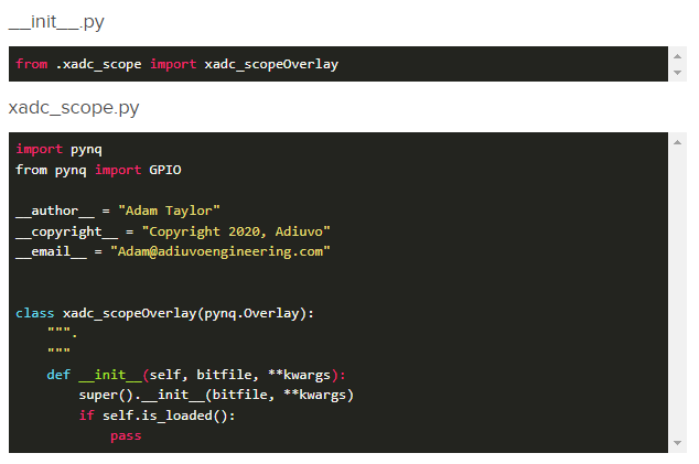
It doesn't do much. I'm wondering if this is a legacy way to prepare overlay load, or if it's really needed.
For the moment, I've kept it as explained by Adam, and it works.
Place the bit- and hwh file from previous blog in a ~/pynq/overlays/xadc_scope folder, together with the two Python files above. rename both to xadc_scope.*.
You don't need to type. The code is available on Adam's hackster.io post.
Prepare Hardware
I'm using a function generator to generate a test signal. It has to be between 0 and 1 V.
In my setup, I used a sinus of 16 kHz, between 148 mV and 554 mV
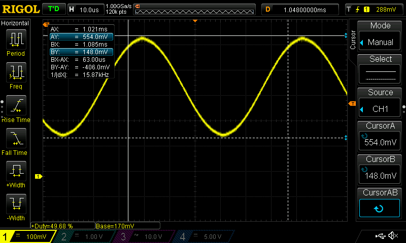
The dedicated analogue input of the Zynq is used, on connector J5:
| J5.GND | function generator ground |
| J5.Vn | function generator ground |
| J5.Vp | function generator signal |
Don't turn the generator on before the PYNQ-Z2 is powered on.
Because we're using PYNQ and Linux, the boot jumper JP1 needs to be placed back to the SD Card position, the card needs to be entered and the network cable plugged in.
Jupyter Notebook and Results
I'm using screen captures here. The blog of Adam has the source code.
First step is to load the bitfile and prime the DMA and memory buffer.
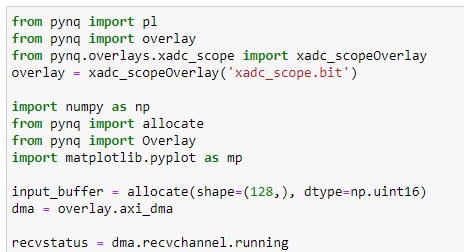
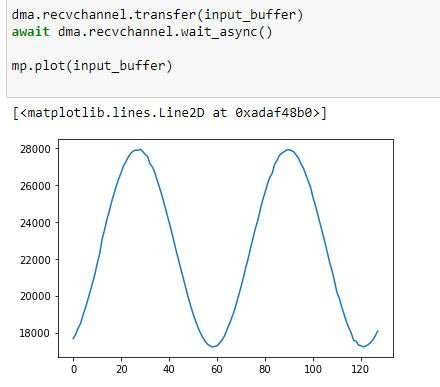
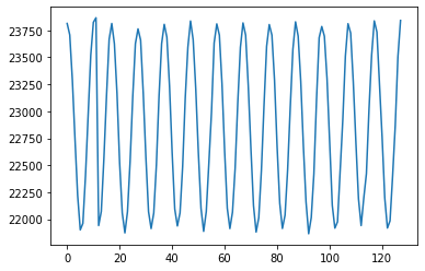
The design is running. We can retrieve a buffer of data and plot it.
You can repeat this step as often as you want.
When you're finished, mop op the allocated memory

To close this post, a capture of a 100 kHz signal, same amplitude
Thank you for reading.

-

yepe
-
Cancel
-
Vote Up
0
Vote Down
-
-
Sign in to reply
-
More
-
Cancel
-

Jan Cumps
in reply to yepe
-
Cancel
-
Vote Up
0
Vote Down
-
-
Sign in to reply
-
More
-
Cancel
Comment-

Jan Cumps
in reply to yepe
-
Cancel
-
Vote Up
0
Vote Down
-
-
Sign in to reply
-
More
-
Cancel
Children